1.4. Migrating from SAS to R: A Skill Conversion Guide
1.4.3 SET in SAS vs. bind_rows() in R
How They Work Under the Hood
SAS SET: - Reads datasets row by row into the Program Data Vector (PDV). - Supports stacking, ordering, flagging source data, and transformations during read. - Missing columns are added with default missing values (. for numeric, blank for character).
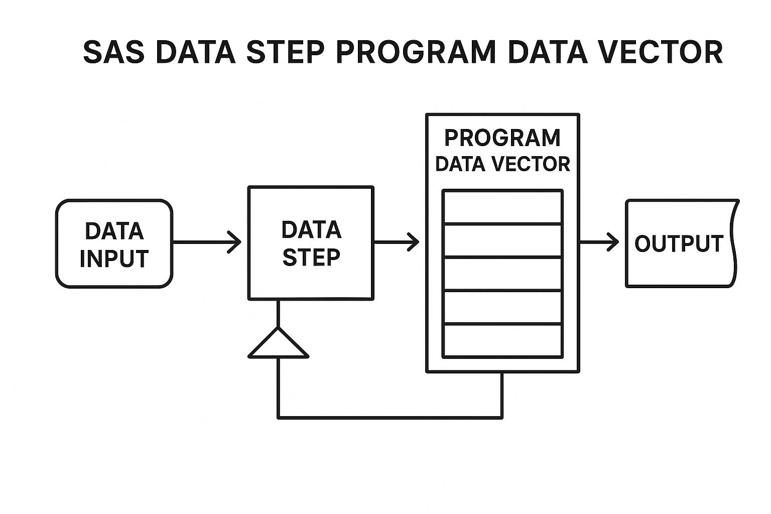
SAS Data Step Program Data Vector (PDV) workflow illustration
Key Characteristics:
- Sequential Processing: Reads datasets row-by-row, minimizing memory usage.
- Automatic Variable Alignment: Handles missing columns by adding them with default missing values.
- Built-in Type Coercion: Performs automatic type conversion with warnings.
- Conditional Processing: Supports complex logic during data reading.
- Source Tracking: Uses
in=option to identify dataset origins.
R bind_rows() (from dplyr): - Appends rows from multiple data frames into one. - Aligns columns by name; adds missing columns with NA. - Supports tracking dataset origin via .id, and can pipe transformations with mutate() and filter().
.png)
Key Characteristics:
- Memory-Based Operations: Loads entire datasets into memory for processing.
- Column Alignment: Automatically aligns columns by name, filling missing ones with
NA. - Strict Type Checking: Prevents silent errors through rigorous validation.
- Explicit Source Tracking: Uses
.idparameter for dataset identification. - Pipeline Integration: Works seamlessly with dplyr chains.
- Comprehensive Error Messages: Provides detailed information about type mismatches.
**Performance Analysis and Benchmarking**
Based on extensive research across multiple sources, performance varies significantly depending on dataset size and use case:
- SAS PROC APPEND: Excellent for simple concatenation.
- R bind_rows(): Good performance with better readability.
Large Datasets (> 1GB):
- SAS SET: Consistent performance regardless of size, optimized for disk I/O.
- SAS PROC APPEND: Most efficient for appending to existing datasets.
- R data.table: Excellent scalability with proper memory management.
**Feature-by-Feature Comparison Table**
| Feature or Use Case | SAS SET |
R bind_rows() (dplyr) |
Key Difference or Note |
|---|---|---|---|
| Copy a dataset | data new; set old; run; |
new <- old |
SAS copies row-by-row; R creates a reference unless reassigned. |
| Stack datasets vertically | set ds1 ds2; |
bind_rows(ds1, ds2) |
Both align by column names. |
| Handle mismatched columns | Adds missing variables automatically with . |
Fills missing with NA |
R is more explicit; can warn on type coercion. |
| Track source dataset | in= + conditional flag assignment |
.id parameter to bind_rows() |
R is more concise and readable. |
| Sort during stack | Requires proc sort then BY clause |
Use arrange() after binding |
SAS enforces presorting; R supports post-processing. |
| Filter rows before binding | where= or if logic in DATA step |
filter() applied before binding |
Filtering can be done inline in both. |
| Derive new variables while stacking | Add variables directly in DATA step logic |
Use mutate() within or before bind_rows() |
R supports column-wise transformations within pipe chains. |
| Interleaving records | Sort both datasets then use BY |
Use arrange() after bind_rows() |
SAS requires physical sort upfront. |
| Data audit traceability | Add manual flags using in= or macro variables |
.id or add metadata columns via mutate() |
R can trace input source more seamlessly with labels. |
Examples with Detailed Execution Flow
1. Copying a Dataset
SAS:
data patients_copy;
  set patients;
run;
- Creates a new dataset
patients_copy. - Reads each row from
patientsinto the PDV. - Writes each unchanged row into the new dataset.
R:
patients_copy <- patients
- Assigns a reference to the original object.
- If you mutate
patients_copy, it may affectpatients. - Use
patients_copy <- dplyr::as_tibble(patients)for safe duplication.
2. Stacking Datasets with Uneven Columns
Scenario: visit1 has Glucose; visit2 has Cholesterol.
SAS:
data visits_all;
  set visit1 visit2;
run;
- SAS builds a variable list from both datasets.
- Adds missing columns automatically.
- Missing values appear as
.in final output.
Example Input:
visit1
| PatientID | VisitDate | Glucose |
|---|---|---|
| 201 | 2023-01-01 | 95 |
| 202 | 2023-01-02 | 103 |
visit2
| PatientID | VisitDate | Cholesterol |
|---|---|---|
| 201 | 2023-02-01 | 180 |
| 203 | 2023-02-02 | 190 |
Expected Output:
| PatientID | VisitDate | Glucose | Cholesterol |
|---|---|---|---|
| 201 | 2023-01-01 | 95 | NA / . |
| 202 | 2023-01-02 | 103 | NA / . |
| 201 | 2023-02-01 | NA / . | 180 |
| 203 | 2023-02-02 | NA / . | 190 |
R:
library(dplyr)

visit1 <- data.frame(
  PatientID = c(201, 202),
  VisitDate = as.Date(c("2023-01-01", "2023-01-02")),
  Glucose = c(95, 103)
)
visit2 <- data.frame(
  PatientID = c(201, 203),
  VisitDate = as.Date(c("2023-02-01", "2023-02-02")),
  Cholesterol = c(180, 190)
)

visits_all <- bind_rows(visit1, visit2)
print(visits_all)
- R aligns columns by name.
- Adds missing columns with
NA. - Can alert on inconsistent data types (e.g., factors vs. characters).
3. Sorting After Stacking / Interleaving by Key
SAS:
proc sort data=visit1; by PatientID; run;
proc sort data=visit2; by PatientID; run;

data interleaved;
  set visit1 visit2;
  by PatientID;
run;
- Requires both datasets to be physically sorted.
- The
BYstatement interleaves rows byPatientID. - Useful for time series or chronological output.
Expected Output:
| PatientID | VisitDate | Glucose | Cholesterol |
|---|---|---|---|
| 201 | 2023-01-01 | 95 | NA / . |
| 201 | 2023-02-01 | NA / . | 180 |
| 202 | 2023-01-02 | 103 | NA / . |
| 203 | 2023-02-02 | NA / . | 190 |
R:
library(dplyr)

visit1 <- data.frame(
  PatientID = c(201, 202),
  VisitDate = as.Date(c("2023-01-01", "2023-01-02")),
  Glucose = c(95, 103)
)
visit2 <- data.frame(
  PatientID = c(201, 203),
  VisitDate = as.Date(c("2023-02-01", "2023-02-02")),
  Cholesterol = c(180, 190)
)

interleaved <- bind_rows(visit1, visit2) %>%
  arrange(PatientID)
print(interleaved)
- Stacks first, then orders the combined dataframe.
- No need to sort upfront.
4. Tagging Source of Each Row
SAS:
data trial_log;
  set screening(in=a) enrollment(in=b);
  if a then Phase = "Screening";
  else if b then Phase = "Enrollment";
run;
in=sets a Boolean variable for each input dataset.- SAS sets
Phaseaccordingly.
Example Input:
screening
| PatientID | Status |
|---|---|
| 301 | Eligible |
| 302 | Ineligible |
enrollment
| PatientID | Status |
|---|---|
| 303 | Enrolled |
| 304 | Withdrawn |
Expected Output:
| PatientID | Status | Phase |
|---|---|---|
| 301 | Eligible | Screening |
| 302 | Ineligible | Screening |
| 303 | Enrolled | Enrollment |
| 304 | Withdrawn | Enrollment |
R:
library(dplyr)

screening <- data.frame(
  PatientID = c(301, 302),
  Status = c("Eligible", "Ineligible")
)
enrollment <- data.frame(
  PatientID = c(303, 304),
  Status = c("Enrolled", "Withdrawn")
)

trial_log <- bind_rows(
  Screening = screening,
  Enrollment = enrollment,
  .id = "Phase"
)
print(trial_log)
.id = "Phase"adds a column with values "Screening" or "Enrollment".- Elegant and traceable.
5. Filtering While Binding
SAS:
data filtered;
  set lab1(where=(ALT > 50)) lab2(where=(ALT > 50));
run;
- Filters rows on input.
where=avoids loading unwanted rows into PDV.
Example Input:
lab1
| PatientID | ALT |
|---|---|
| 401 | 45 |
| 402 | 78 |
lab2
| PatientID | ALT |
|---|---|
| 403 | 85 |
| 404 | 42 |
Expected Output:
| PatientID | ALT |
|---|---|
| 402 | 78 |
| 403 | 85 |
R:
library(dplyr)

lab1 <- data.frame(
  PatientID = c(401, 402),
  ALT = c(45, 78)
)
lab2 <- data.frame(
  PatientID = c(403, 404),
  ALT = c(85, 42)
)

filtered <- bind_rows(
  filter(lab1, ALT > 50),
  filter(lab2, ALT > 50)
)
print(filtered)
- Applies logical filters before stacking.
- Keeps memory footprint smaller.
6. Deriving Variables Inline During Binding
SAS:
data enriched;
  set siteA(in=a) siteB(in=b);
  if a then Region = "East";
  else if b then Region = "West";
  VisitMonth = month(VisitDate);
run;
- Derives
Regionbased on source. - Calculates
VisitMonthdynamically during row processing.
Example Input:
siteA
| PatientID | VisitDate |
|---|---|
| 501 | 2023-01-15 |
| 502 | 2023-02-20 |
siteB
| PatientID | VisitDate |
|---|---|
| 503 | 2023-01-10 |
| 504 | 2023-03-05 |
Expected Output:
| PatientID | VisitDate | Region | VisitMonth |
|---|---|---|---|
| 501 | 2023-01-15 | East | 1 |
| 502 | 2023-02-20 | East | 2 |
| 503 | 2023-01-10 | West | 1 |
| 504 | 2023-03-05 | West | 3 |
R:
library(dplyr)
library(lubridate)

siteA <- data.frame(
  PatientID = c(501, 502),
  VisitDate = as.Date(c("2023-01-15", "2023-02-20"))
)
siteB <- data.frame(
  PatientID = c(503, 504),
  VisitDate = as.Date(c("2023-01-10", "2023-03-05"))
)

enriched <- bind_rows(
  mutate(siteA, Region = "East", VisitMonth = lubridate::month(VisitDate)),
  mutate(siteB, Region = "West", VisitMonth = lubridate::month(VisitDate))
)
print(enriched)
- Adds source identifier and month in a single pipeline.
- Clean, expressive, and efficient.
7. Error Handling Scenarios in R
Common Error Types and Solutions
1. Type Mismatch Errors:
library(dplyr)
library(purrr)

# Problem: Mixed data types in ID columns
df1 <- data.frame(ID = c("A001", "A002"), value = c(10, 20))
df2 <- data.frame(ID = c(1, 2), value = c(30, 40))

# Solution: Type standardization
df1 <- df1 %>% mutate(ID = as.character(ID))
df2 <- df2 %>% mutate(ID = as.character(ID))
result <- bind_rows(df1, df2)
Output:
    ID value
1 A001    10
2 A002    20
3    1    30
4    2    40
R Explanation
- Problem: Attempting to bind data frames with mismatched ID types (character vs numeric).
- Solution: Use
mutate()withacross()to standardize ID types before binding. - Output: Successfully binds rows with consistent ID types, avoiding type mismatch errors.
2. Column Name Mismatches:
library(dplyr)
library(purrr)

df1 <- data.frame(ID = c("A001", "A002"), value = c(10, 20))
df2 <- data.frame(ID2 = c("A003", "A004"), value2 = c(30, 40))

# Rename columns safely
df1_renamed <- df1 %>% rename(ID = any_of(c("ID", "ID2")),
                value = any_of(c("value", "value2")))
df2_renamed <- df2 %>% rename(ID = any_of(c("ID", "ID2")),
                value = any_of(c("value", "value2")))

result <- bind_rows(df1_renamed, df2_renamed)
print(result)
Output:
> result <- safe_bind_names(df1, df2)
> print(result)
    ID value
1 A001    10
2 A002    20
3 A003    30
4 A004    40
R Explanation
- Problem: Attempting to bind data frames with different column names.
- Solution: Use
rename()to standardize column names before binding. - Output: Successfully binds rows with consistent column names, avoiding binding errors.
3. Duplicate Rows:
library(dplyr)
library(purrr)
# Problem: Duplicate rows in datasets
df1 <- data.frame(ID = c("A001", "A002"), value = c(10, 20))
df2 <- data.frame(ID = c("A001", "A003"), value = c(10, 30))
# Solution: Remove duplicates after binding
result <- bind_rows(df1, df2) %>% distinct()
Output:
> result
    ID value
1 A001    10
2 A002    20
3 A003    30
R Explanation
- Problem: Attempting to bind data frames with potential duplicate rows.
- Solution: Use
distinct()to remove duplicate rows after binding. - Output: Successfully binds rows and removes duplicates, ensuring unique entries.
**Resource download links**
1.4.3.-SET-in-SAS-vs-bind_rows-in-R.zip