1.5. SAS PROCEDURES -> Equivalent in R
1.5.2. PROC FREQ - frequency analysis in SAS and R
Produce summaries of grade distribution:
- Overall frequency
- By department
- Cross-tab by department & gender
- Percentages within group
- Cumulative insights, pivoting, and formatting
Input Table: students
We’ll assume the following dataset for both SAS and R:
| DEPT | GENDER | GRADE |
|---|---|---|
| Math | M | A |
| Math | F | A |
| Math | M | B |
| Math | M | B |
| Math | F | C |
| Physics | F | A |
| Physics | M | B |
| Physics | F | C |
| Physics | F | A |
| Biology | M | A |
| Biology | F | A |
| Biology | M | B |
| Biology | F | B |
| Biology | F | A |
| Biology | F | C |
1. Overall Frequency of GRADE
Goal Count how many students got A, B, or C—across all departments.
SAS Code
proc freq data=students;
  tables grade;
run;
proc freq: Launches the frequency procedure.tables grade;: Requests frequency counts for the GRADE column.- The output includes counts, percentages, cumulative counts and percentages.
R Code
students <- tibble::tibble(
  DEPT = c("Math", "Math", "Math", "Math", "Math", "Physics", "Physics", "Physics", "Physics", "Biology", "Biology", "Biology", "Biology", "Biology", "Biology"),
  GENDER = c("M", "F", "M", "M", "F", "F", "M", "F", "F", "M", "F", "M", "F", "F", "F"),
  GRADE = c("A", "A", "B", "B", "C", "A", "B", "C", "A", "A", "A", "B", "B", "A", "C")
)
students %>% count(GRADE)
count(GRADE): Counts how many times each GRADE value appears.
Output
| GRADE | Count |
|---|---|
| A | 6 |
| B | 4 |
| C | 2 |
2. Grade Frequency by Department
Goal Get grade distribution within each department.
SAS Code
proc sort data=students; by dept;

proc freq data=students noprint;
  by dept;
  tables grade / out=grade_by_dept(drop=percent);
run;
proc sort: Required before usingBY dept;inPROC FREQ.noprint: Suppresses printed output and sends results to a dataset.out=...: Saves the count output; we drop PERCENT here.
R Code
students %>%
  group_by(DEPT) %>%
  count(GRADE, name = "Count")
group_by(DEPT): Sets department as the grouping key.count(GRADE): Within each department, count how often each grade appears.name = "Count": Renames the defaultncolumn for readability.
Output
| DEPT | GRADE | Count |
|---|---|---|
| Math | A | 2 |
| Math | B | 2 |
| Math | C | 1 |
| Physics | A | 2 |
| Physics | B | 1 |
| Physics | C | 1 |
| Biology | A | 3 |
| Biology | B | 2 |
| Biology | C | 1 |
3. Cross-tabulation: GRADE × GENDER within DEPT
Goal See how many males/females got each grade in each department.
SAS Code
proc freq data=students noprint;
  by dept;
  tables grade*gender / out=cross_tab(drop=percent);
run;
grade*gender: Requests cross-tab between GRADE and GENDER.- Grouping still applies to each DEPT due to
BY dept.
R Code
students %>%
  group_by(DEPT) %>%
  count(GRADE, GENDER, name = "Count")
count(GRADE, GENDER): Creates 2D frequency tables per department.
Output
| DEPT | GRADE | GENDER | Count |
|---|---|---|---|
| Math | A | M | 1 |
| Math | A | F | 1 |
| Math | B | M | 2 |
| Math | C | F | 1 |
| Physics | A | F | 2 |
| Physics | B | M | 1 |
| Physics | C | F | 1 |
| Biology | A | M | 1 |
| Biology | A | F | 2 |
| Biology | B | M | 1 |
| Biology | B | F | 1 |
| Biology | C | F | 1 |
4. Add Percentages within Group
Goal Include what percent of each department received each grade.
R Code
students %>%
  group_by(DEPT) %>%
  count(GRADE, name = "Count") %>%
  mutate(Percent = round(Count / sum(Count) * 100, 1))
mutate(...): Adds a new columnPercent.Count / sum(Count): Proportion of each grade within its department.round(..., 1): Keep results clean to 1 decimal place.
Output
| DEPT | GRADE | Count | Percent |
|---|---|---|---|
| Math | A | 2 | 40.0 |
| Math | B | 2 | 40.0 |
| Math | C | 1 | 20.0 |
| Physics | A | 2 | 50.0 |
| Physics | B | 1 | 25.0 |
| Physics | C | 1 | 25.0 |
| Biology | A | 3 | 50.0 |
| Biology | B | 2 | 33.3 |
| Biology | C | 1 | 16.7 |
5. Cumulative Metrics (Optional)
students %>%
  group_by(DEPT) %>%
  count(GRADE, name = "Count") %>%
  arrange(DEPT, desc(Count)) %>%
  mutate(
    Percent = round(Count / sum(Count) * 100, 1),
    CumCount = cumsum(Count),
    CumPercent = round(cumsum(Count) / sum(Count) * 100, 1)
  )
arrange(desc(Count)): Sort grades by most common per department.cumsum(Count): Builds cumulative totals.CumPercent: Useful for Pareto analysis or targeting thresholds.
6. Wide Format for Reporting
library(tidyr)

students %>%
  count(DEPT, GRADE) %>%
  pivot_wider(names_from = GRADE, values_from = n, values_fill = 0)
pivot_wider(): Converts long → wide format for tabular reports.values_fill = 0: Ensures missing values show as 0.
Output
| DEPT | A | B | C |
|---|---|---|---|
| Biology | 3 | 2 | 1 |
| Math | 2 | 2 | 1 |
| Physics | 2 | 1 | 1 |
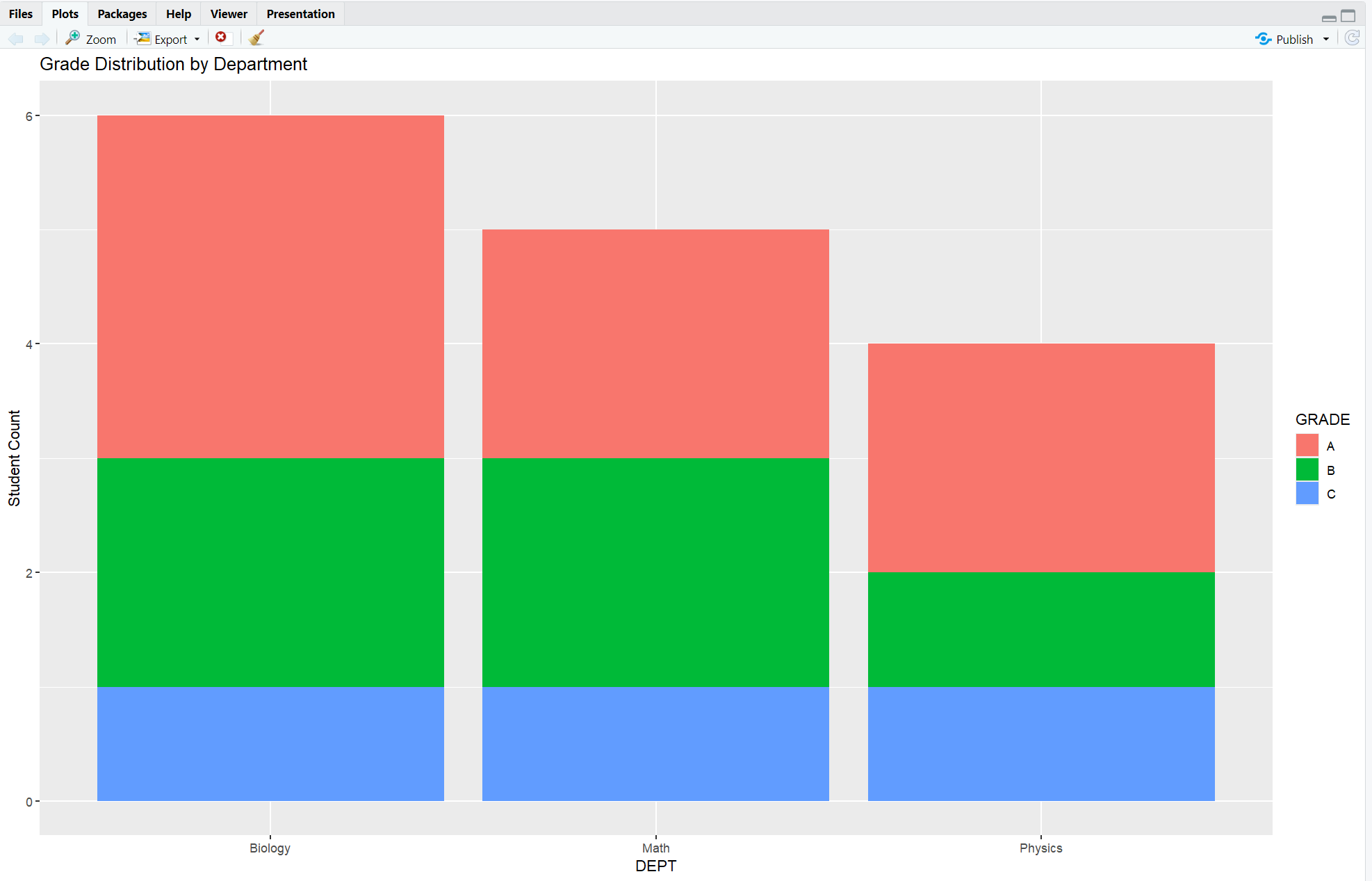
7. Visualization: Stacked Bar Chart
library(ggplot2)

students %>%
  count(DEPT, GRADE) %>%
  ggplot(aes(x = DEPT, y = n, fill = GRADE)) +
  geom_col(position = "stack") +
  labs(title = "Grade Distribution by Department", y = "Student Count")
geom_col()uses pre-counted data.fill = GRADEstacks by grade per department.- Helpful for presentations and spotting trends visually.
Output:
**Summary Table: SAS vs R**
| Feature | SAS (PROC FREQ) |
R (dplyr::count() + friends) |
|---|---|---|
| 1-way Frequency | tables var; |
count(var) |
| 2-way Grouped Count | BY var; tables var2; |
group_by(var1) %>% count(var2) |
| Cross-tab | tables var1*var2; |
count(var1, var2) |
| Percentages | Built-in | mutate(percent = n / sum(n)) |
| Cumulative stats | Custom logic | Easy with cumsum() |
| Pivot for reporting | Manual PROC TABULATE/TABLE | pivot_wider() |
| Visuals | External (e.g., PROC SGPLOT) | Native with ggplot2 |
**Resource download links**
1.5.2.-PROC-FREQ-frequency-analysis-in-SAS-and-R.zip
⁂