2.4.2. Dates and Times in R: lubridate & hms
1. Introduction
Based on the comprehensive exploration of the Atorus Research Academy e-learning content, I have created an extensive tutorial covering the lubridate and hms packages for R programming in clinical applications. This guide significantly enhances the original material with additional examples, error handling scenarios, and advanced applications.
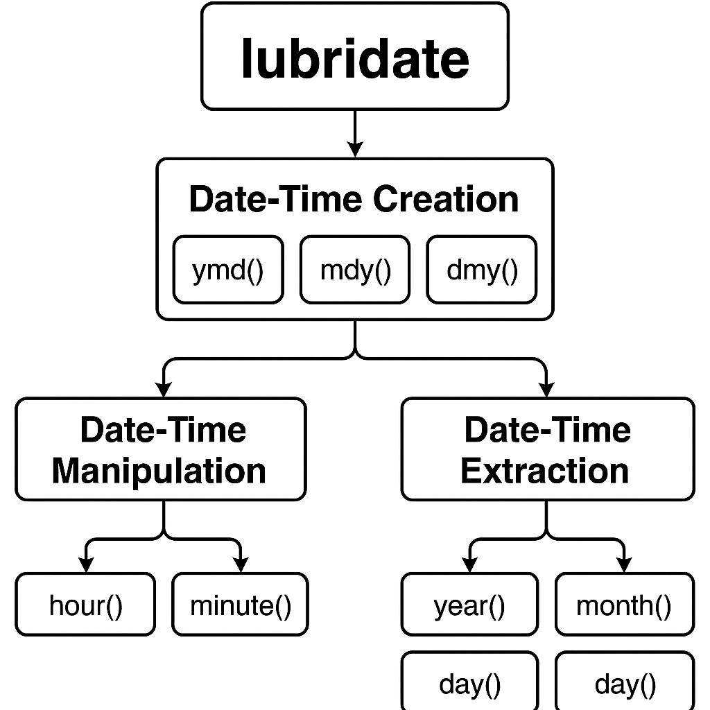
Lubridate package workflow diagram for R programming
2. Core Data Types and Concepts
R handles temporal data through three primary data types that serve different purposes in clinical programming:[^2]
Date Objects store dates without time information as the number of days since January 1, 1970. These are ideal for visit dates, enrollment dates, and other calendar-based clinical events.
Date-Time Objects (POSIXct) combine date and time information, stored as seconds since the Unix epoch, and include timezone awareness. These are essential for precise timestamp recording in clinical trials.
Time Objects (hms) represent time-of-day values as durations since midnight, perfect for dosing times, procedure schedules, and time-based measurements.
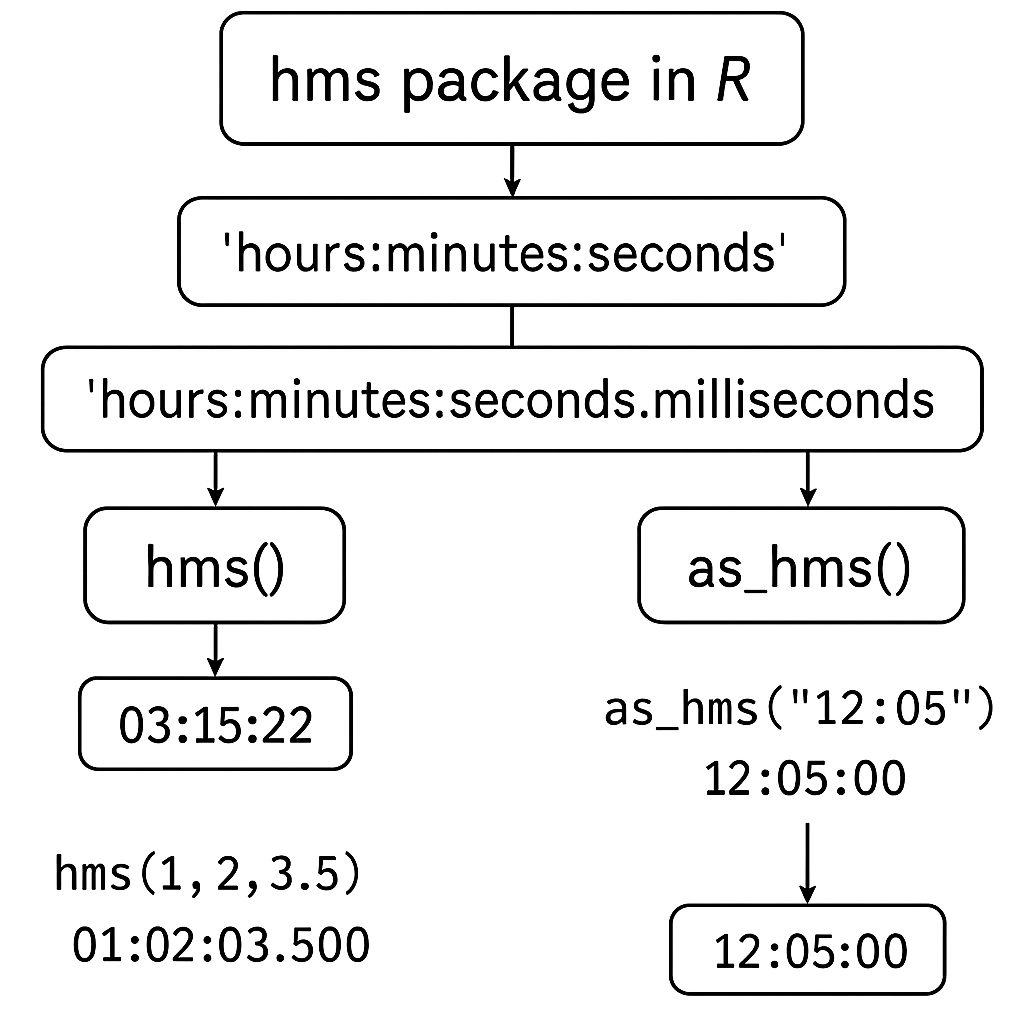
HMS package time format diagram for R programming
3. Creating Dates and Date-Times
The lubridate package provides multiple approaches for creating date-time objects, each optimized for different data scenarios commonly encountered in clinical programming.[^1][^3]
Parsing Functions: The Recommended Approach
The most intuitive method uses parsing functions named after the order of date components:
# Year-Month-Day formats
ymd("2022-01-15")
ymd_hms("2022-01-15 10:30:45")

# Month-Day-Year formats
mdy("01/15/2022")
mdy_hms("01/15/2022 10:30:45")

# Day-Month-Year formats
dmy("15-01-2022")
dmy_hms("15-01-2022 10:30:45")
These functions are separator agnostic, meaning they work with various delimiters (dashes, slashes, spaces) and can even parse flexible text formats like "January 4th 2022".[^1][^3]
Converting from Different Input Types
The as_datetime() and as_date() functions handle conversion from numeric Unix timestamps, existing date objects, and character strings with specific format specifications:
# From Unix timestamp
as_datetime(1641040230)

# From character with format specification
as_datetime("02-17-2022 08:25:30", format = "%m-%d-%Y %H:%M:%S")
Creating from Individual Components
For datasets where date components are stored in separate columns (common in clinical databases), the make_datetime() and make_date() functions provide clean solutions:
make_datetime(year = 2022, month = 12, day = 13,
              hour = 10, min = 44, sec = 30)
make_date(year = 2022, month = 12, day = 13)
4. Working with Times Using HMS
The hms package specializes in handling time-of-day values, which are crucial for clinical applications requiring precise timing:[^2][^4]
# From character (requires colon separators)
hms::as_hms("09:30:45")

# From numeric seconds since midnight
hms::as_hms(34245)  # Results in 09:30:45

# From components
hms::hms(hours = 9, minutes = 30, seconds = 45)
Important Note: Unlike lubridate functions, hms requires proper colon separators and is not separator agnostic.
5. Date and Time Arithmetic
One of lubridate's most powerful features is its sophisticated approach to temporal arithmetic, addressing the complexities of calendar systems and time zones.[^1][^5][^6]
Difftimes: Basic Time Differences
Simple subtraction between date objects creates difftime objects that automatically handle unit conversion:
start_date <- as_date("2019-03-26")
end_date <- as_date("2019-09-24")
duration <- end_date - start_date  # Results in 182 days
Durations vs. Periods: A Critical Distinction
Durations represent exact amounts of time in seconds and are suitable when physical time matters:
dyears(1)    # Exact number of seconds in a year
dmonths(3)   # Exact number of seconds in 3 months
Periods represent calendar time and handle irregularities like leap years and varying month lengths:
years(1)     # Calendar period of 1 year
months(3)    # Calendar period of 3 months
The distinction is crucial for clinical applications:
# Leap year example
leap_date <- as_date("2020-01-01")
leap_date + dyears(1)  # Results in "2020-12-31" (duration)
leap_date + years(1)   # Results in "2021-01-01" (period)
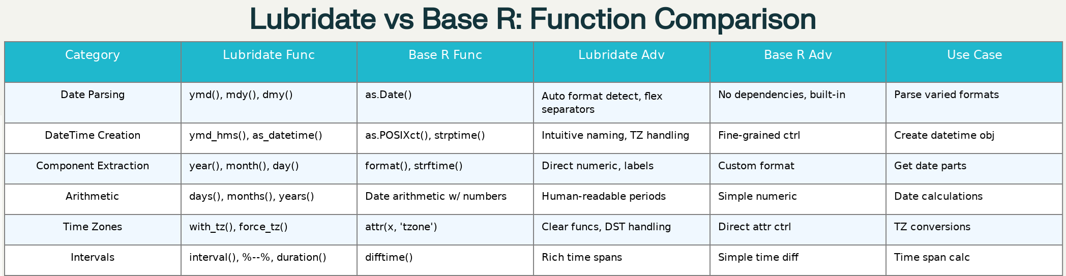
Comprehensive comparison of lubridate vs base R date-time functions
6. Extracting Date and Time Components
Lubridate provides comprehensive functions for extracting temporal components, essential for creating derived variables in clinical datasets:[^1][^6]
sample_datetime <- ymd_hms("2019-06-26 11:45:57")

# Date components
year(sample_datetime)      # 2019
month(sample_datetime)     # 6
day(sample_datetime)       # 26
wday(sample_datetime)      # 4 (Wednesday)

# Time components
hour(sample_datetime)      # 11
minute(sample_datetime)    # 45
second(sample_datetime)    # 57

# With labels for reporting
month(sample_datetime, label = TRUE)  # "Jun"
wday(sample_datetime, label = TRUE)   # "Wed"
7. Clinical Programming Applications
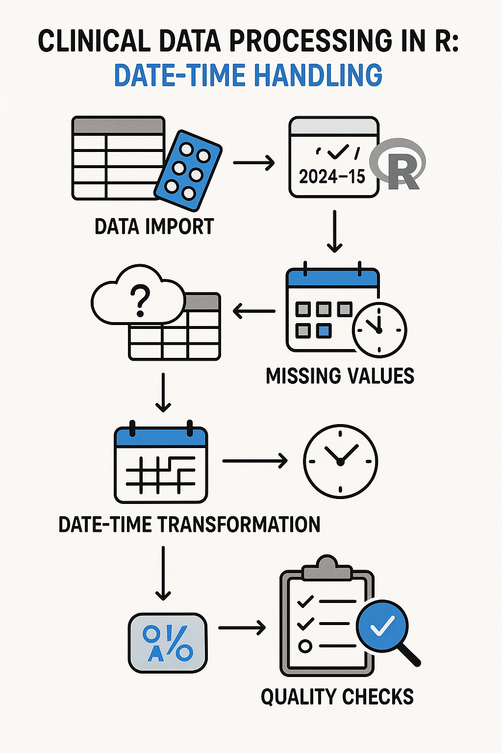
Clinical data processing flowchart with R date-time handling
Study Day Calculations
A fundamental requirement in clinical programming is calculating study days relative to a baseline date:
baseline_date <- ymd("2022-01-01")
visit_date <- ymd("2022-02-15")
study_day <- as.numeric(visit_date - baseline_date) + 1  # 46
Adverse Event Duration Analysis
Clinical trials require precise tracking of adverse event durations:
ae_start <- ymd("2022-01-20")
ae_end <- ymd("2022-01-25")
ae_duration <- as.numeric(ae_end - ae_start) + 1  # 6 days

# Classification based on duration
ae_severity <- case_when(
  ae_duration <= 1 ~ "Mild",
  ae_duration <= 3 ~ "Moderate",
  TRUE ~ "Severe"
)
Time Window Calculations
Clinical protocols often specify time windows for procedures and assessments:
# Calculate visit windows
scheduled_date <- ymd("2022-03-15")
window_start <- scheduled_date - days(3)
window_end <- scheduled_date + days(3)

# Check if actual visit falls within window
actual_visit <- ymd("2022-03-17")
in_window <- actual_visit >= window_start & actual_visit <= window_end
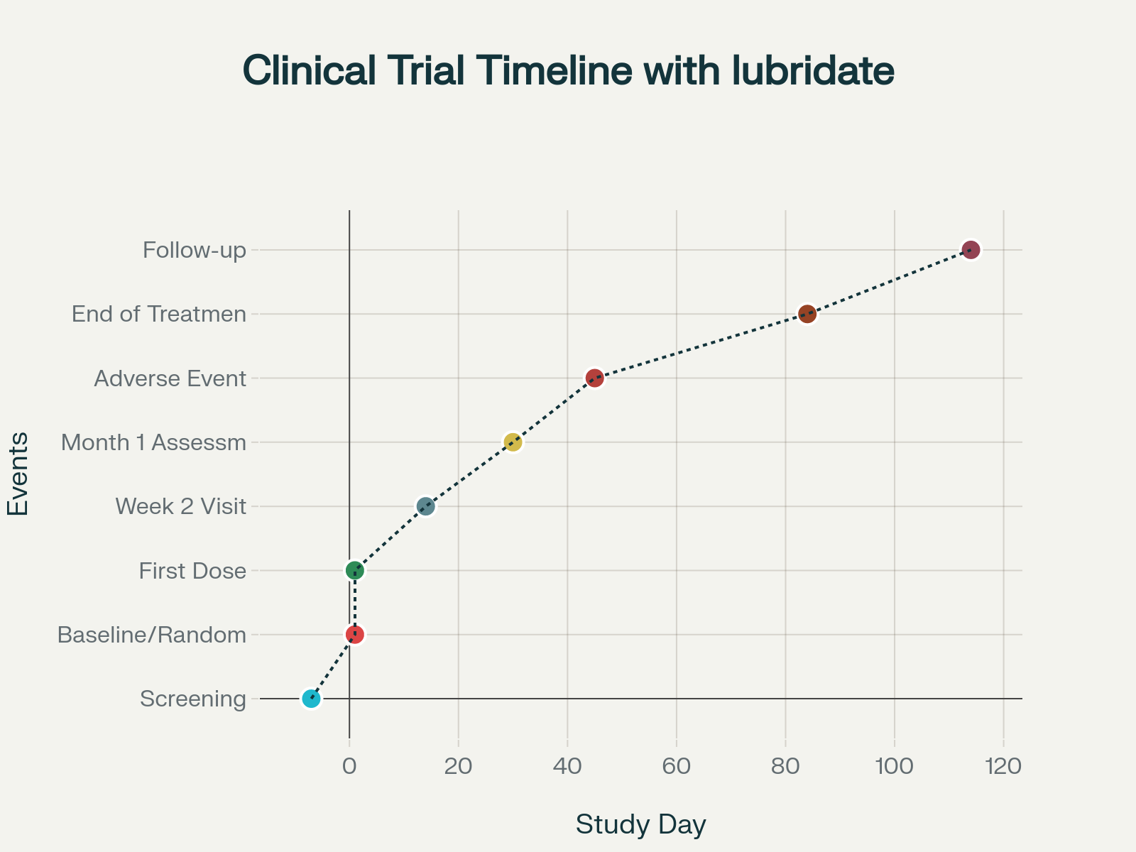
Clinical trial timeline with lubridate function usage examples
8. Error Handling and Best Practices
Robust Date Parsing
Clinical data often contains inconsistent date formats. A robust parsing function handles multiple scenarios:
safe_date_parse <- function(date_string) {
  # Try base R formats first
  base_formats <- c("%Y-%m-%d", "%m/%d/%Y", "%d-%m-%Y", "%Y%m%d")

  for (fmt in base_formats) {
    result <- tryCatch(as.Date(date_string, format = fmt),
                      error = function(e) NULL)
    if (!is.null(result) && !is.na(result)) return(result)
  }

  # Try lubridate functions
  lubridate_funcs <- list(ymd, mdy, dmy, ydm, myd, dym)
  for (func in lubridate_funcs) {
    result <- tryCatch(func(date_string),
                      warning = function(w) NULL,
                      error = function(e) NULL)
    if (!is.null(result) && !is.na(result)) return(result)
  }

  return(NA)
}
Handling Partial Dates
Clinical data sometimes contains partial dates (e.g., "2022-06-UNK"):
handle_partial_date <- function(date_str) {
  # Replace unknown day with middle of month
  date_str <- gsub("-UNK$", "-15", date_str)

  # Use truncated parameter for missing components
  ymd(date_str, truncated = 2)
}
Timezone Management
Clinical trials often span multiple time zones. Proper timezone handling is essential:
# Create datetime with specific timezone
utc_time <- ymd_hms("2022-12-25 10:30:00", tz = "UTC")

# Convert to different timezone (changes the time)
local_time <- with_tz(utc_time, "America/New_York")

# Force timezone without conversion (keeps same time)
forced_time <- force_tz(utc_time, "America/New_York")
9. Advanced Features and Performance Considerations
Vectorized Operations
Lubridate functions are vectorized for efficient processing of large datasets:
# Efficient: Process entire vectors at once
date_vector <- c("2022-01-01", "2022-01-02", "2022-01-03")
parsed_dates <- ymd(date_vector)

# Less efficient: Individual processing
parsed_individual <- sapply(date_vector, ymd)
Memory Efficiency for Large Datasets
For clinical datasets with millions of records, consider using data.table for memory efficiency:
library(data.table)
large_dt <- data.table(date_char = rep("2022-01-01", 1000000))
large_dt[, date_parsed := ymd(date_char)]  # Efficient in-place operation
10. Integration with Tidyverse Workflows
Lubridate seamlessly integrates with dplyr and other tidyverse packages for comprehensive data processing:
clinical_data %>%
  mutate(
    visit_date = ymd(visit_date_char),
    visit_month = lubridate::month(visit_date, label = TRUE),
    study_day = as.numeric(visit_date - baseline_date) + 1,
    study_week = ceiling(study_day / 7)
  ) %>%
  filter(study_day <= 84) %>%
  group_by(study_week) %>%
  summarise(avg_lab_value = mean(lab_value, na.rm = TRUE))
11. Summary and Recommendations
The lubridate and hms packages provide a comprehensive toolkit for handling temporal data in R, with particular strengths in clinical programming applications. Key recommendations include:
- Use parsing functions (
ymd(),mdy(), etc.) for character data conversion - Implement robust error handling for inconsistent data formats
- Understand the distinction between periods and durations
- Be explicit about timezone handling in multi-site studies
- Leverage vectorization for performance with large datasets
- Document temporal assumptions and conventions in your code
The enhanced tutorial materials provide a complete foundation for implementing professional-grade temporal data processing in clinical programming contexts, with comprehensive error handling, best practices, and real-world examples that extend well beyond the basics covered in the original e-learning content.