1. R Fundamentals
1.2 Getting Started with R Programming
- Introduction to R Programming:
- R is a language designed for statistical computing and graphics.
- Understanding its data structures is essential for efficient data analysis and manipulation.
1.2.2 Data Structures (Objects) in R
- What are Data Structures in R?
- Data structures are ways to organize and store data for efficient access and modification.
- R provides several built-in structures, each suited for different types of data and operations.
Overview of Core Structures
- Dimensionality vs. Homogeneity:
- R classifies data structures by their number of dimensions (1D, 2D, ND) and whether they hold only one type of data (homogeneous) or multiple types (heterogeneous).
- The chart below visually compares these structures.
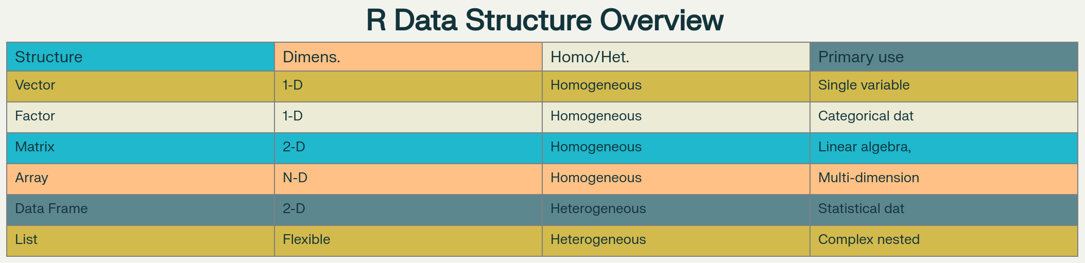
R Data Structures Comparison Chart
- 1-D homogeneous – atomic vectors (numeric, character, logical, integer, complex)
- 1-D heterogeneous – lists (can nest any object)
- 2-D homogeneous – matrices (all elements same type)
- 2-D heterogeneous – data frames & tibbles (mixed column types)
- N-D homogeneous – arrays (3-D, 4-D, multi-dimensional)
- Factors – specialized 1-D categorical vectors with predefined levels
1. Vectors
- Vectors in R:
- The most basic data structure in R, holding elements of the same type (numeric, character, logical, etc.).
- All operations in R are vectorized, meaning they apply to entire vectors at once.
Creating and Basic Operations
- Creating Vectors:
c()combines values into a vector.- Named vectors allow you to assign names to elements for easier access.
- The
:operator creates sequences.
# Multiple creation methods
sales_data <- c(1200, 1500, 980, 2100, 1800) # Numeric vector
quarterly_results <- c(Q1=25000, Q2=31000, Q3=28000, Q4=35000) # Named vector
temperature_range <- -5:10  # Sequence from -5 to 10
Output:

- Explanation:
sales_data <- c(1200, 1500, 980, 2100, 1800)- This creates a numeric vector called
sales_datacontaining five sales figures. - Each value is a separate element in the vector, and all are stored as numbers.
- This creates a numeric vector called
quarterly_results <- c(Q1=25000, Q2=31000, Q3=28000, Q4=35000)- This creates a named numeric vector, where each element is associated with a name (
Q1,Q2, etc.). - You can access values by their names, e.g.,
quarterly_results["Q2"]returns31000.
- This creates a named numeric vector, where each element is associated with a name (
temperature_range <- -5:10- The colon operator
:generates a sequence of integers from -5 to 10 (inclusive). - The resulting vector contains all integer values in that range, useful for generating regular sequences.
- The colon operator
**Common Warning Scenarios**
Mixing Data Types
c(1, "two", 3)- R coerces everything to character, and usually gives no warning —but this can lead to unexpected behavior if you assume it's numeric.
Coercion in Logical Operations
x <- c(TRUE, FALSE, "maybe")- The string forces coercion to character. No warning, but semantic confusion!
Named Vector Mismatches
named_vec <- c(A=1, B=2)
named_vec[c("A","B")]
named_vec[c("A", "C")]
Output:
> named_vec <- c(A=1, B=2) > named_vec A B 1 2 > named_vec[c("A","B")] A B 1 2 > named_vec[c("A", "C")] A <NA> 1 NA- Accessing a nonexistent name (
"C") returnsNAsilently. No warning, but something to watch out for.
- Accessing a nonexistent name (
**Typical Error Triggers**
Out-of-Bounds Indexing
x <- c(5, 10) x[3]- No error, but returns
NA. Error happens if you try to assign to an index that doesn’t exist in a fixed-length structure like a matrix.
- No error, but returns
Wrong Type for Indexing
x <- c(5, 10) x["not_a_name"]- If no such name exists, returns
NA, but some cases (like a NULL or list index) can throw errors.
- If no such name exists, returns
Non-Numeric Operations on a Numeric Vector
x <- c(1, 2, 3) mean("apple")- You'll get an error: “argument is not numeric or logical: returning NA”.
Length Mismatch in Assignment
x <- c(1, 2, 3)
x[] <- c(1, 2)  # Warning: number of items to replace is not a multiple of replacement length
Output:
> x <- c(1, 2, 3)
> x[] <- c(1, 2)  # Warning: number of items to replace is not a multiple of replacement length
Warning message:
In x[] <- c(1, 2) :
  number of items to replace is not a multiple of replacement length
> x
[1] 1 2 1
- This warning occurs because you are trying to replace elements in
xwith a vector of a different length. R will recycle the shorter vector, but it may not be what you intended.
1.1 Vector Math Operations
- Element-wise Operations:
- Arithmetic operations on vectors are performed element by element, without explicit loops.
# Create sample dataset
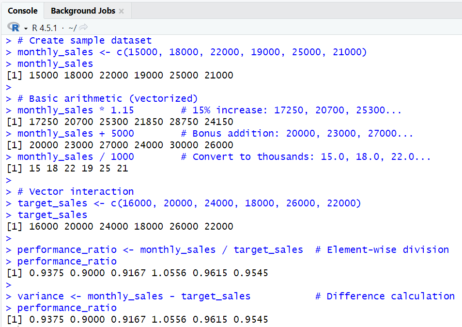
monthly_sales <- c(15000, 18000, 22000, 19000, 25000, 21000)
# Basic arithmetic (vectorized)
monthly_sales * 1.15 # 15% increase: 17250, 20700, 25300...
monthly_sales + 5000 # Bonus addition: 20000, 23000, 27000...
monthly_sales / 1000 # Convert to thousands: 15.0, 18.0, 22.0...
# Vector interaction
target_sales <- c(16000, 20000, 24000, 18000, 26000, 22000)
performance_ratio <- monthly_sales / target_sales # Element-wise division
variance <- monthly_sales - target_sales # Difference calculation
Output:
- Explanation:
monthly_sales <- c(15000, 18000, 22000, 19000, 25000, 21000)- Creates a vector of monthly sales figures for six months.
monthly_sales * 1.15- Multiplies each sales value by 1.15, increasing each by 15%.
- The result is a new vector: each element is the original sales value increased by 15%.
monthly_sales + 5000- Adds 5000 to each element, simulating a bonus or adjustment to every month's sales.
monthly_sales / 1000- Divides each sales value by 1000, converting the numbers to thousands for easier reading or plotting.
target_sales <- c(16000, 20000, 24000, 18000, 26000, 22000)- Creates a vector of target sales for the same six months.
performance_ratio <- monthly_sales / target_sales- Divides each actual sales value by the corresponding target sales value, producing a ratio for each month.
- If the ratio is above 1, the target was exceeded; below 1, the target was missed.
variance <- monthly_sales - target_sales- Subtracts the target sales from the actual sales for each month, showing the difference (positive or negative) for each period.
1.2 Vector Recycling in Practice
- Vector Recycling:
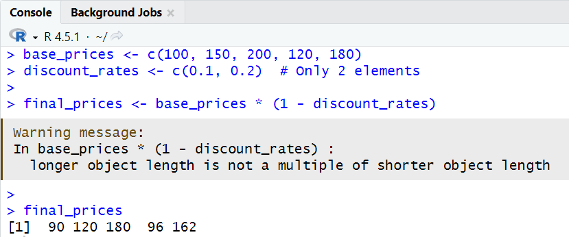
- If two vectors are of unequal length, R repeats (recycles) the shorter one to match the longer vector's length.
base_prices <- c(100, 150, 200, 120, 180)
discount_rates <- c(0.1, 0.2)  # Only 2 elements

# R recycles discount_rates: 0.1, 0.2, 0.1, 0.2, 0.1
final_prices <- base_prices * (1 - discount_rates)
# Result: 90, 120, 180, 96, 162
- Explanation:
base_prices <- c(100, 150, 200, 120, 180)- A vector of five product base prices.
discount_rates <- c(0.1, 0.2)- A vector of two discount rates (10% and 20%).
- When calculating
final_prices, R automatically repeats thediscount_ratesvector to match the length ofbase_prices:- The operation is performed as:
- 100 * (1 - 0.1) = 90
- 150 * (1 - 0.2) = 120
- 200 * (1 - 0.1) = 180
- 120 * (1 - 0.2) = 96
- 180 * (1 - 0.1) = 162
- This demonstrates how R handles operations between vectors of different lengths.
- The operation is performed as:
1.3 Vector Functions
- Common Vector Functions:
- Functions like
sum(),mean(),min(),max(), andwhich.max()operate on entire vectors.
- Functions like
product_ratings <- c(4.2, 3.8, 4.7, 4.1, 3.9, 4.5, 4.3)

sum(product_ratings)         # 29.5
mean(product_ratings)        # 4.214
min(product_ratings)         # 3.8
max(product_ratings)         # 4.7
which.max(product_ratings)   # 3 (position of maximum)
- Explanation:
product_ratingsis a vector of customer ratings for a product.sum(product_ratings)- Adds up all the ratings, giving the total score.
mean(product_ratings)- Calculates the average rating by dividing the sum by the number of ratings.
min(product_ratings)andmax(product_ratings)- Find the lowest and highest ratings in the vector.
which.max(product_ratings)- Returns the index (position) of the highest rating in the vector (here, the 3rd element).
2. Vector Math
- Efficient Computation:
- R's vectorization allows for fast, concise calculations on entire datasets.
**Arithmetic Operations**
- Bulk Calculations:
- Multiplying, adding, or dividing vectors applies the operation to each element.
# E-commerce example
product_costs <- c(25, 40, 15, 60, 35, 20)
markup_multiplier <- 2.5

# Calculate retail prices (vectorized)
retail_prices <- product_costs * markup_multiplier
# Result: 62.5, 100.0, 37.5, 150.0, 87.5, 50.0

# Bulk operations
tax_rate <- 0.08
final_prices <- retail_prices * (1 + tax_rate)
savings <- retail_prices - product_costs
profit_margins <- savings / retail_prices
- Explanation:
retail_prices <- product_costs * markup_multiplier- Calculates retail prices by multiplying each product's cost by the markup factor.
final_prices <- retail_prices * (1 + tax_rate)- Applies tax to each retail price to get the final price.
savings <- retail_prices - product_costs- Calculates the savings (or profit) for each product by subtracting the cost from the retail price.
profit_margins <- savings / retail_prices- Calculates the profit margin for each product as a percentage of the retail price.
**Vector Interaction Examples**
- Logical Comparisons:
- Logical operations return TRUE/FALSE for each element, useful for filtering or flagging data.
# Inventory management
current_stock <- c(45, 23, 67, 12, 89, 34)
reorder_levels <- c(20, 15, 30, 25, 40, 15)

# Determine reorder needs
needs_reorder <- current_stock < reorder_levels  # Logical vector
reorder_quantity <- pmax(0, reorder_levels - current_stock)
- Explanation:
needs_reorder <- current_stock < reorder_levels- Compares current stock levels to reorder levels, returning a logical vector (TRUE/FALSE) indicating which items need reordering.
reorder_quantity <- pmax(0, reorder_levels - current_stock)- Calculates the quantity to reorder for each item, ensuring no negative values (using
pmaxto compare with 0).
- Calculates the quantity to reorder for each item, ensuring no negative values (using
3. Subsetting
- Extracting Data:
- Subsetting allows you to select, exclude, or filter elements from vectors and data frames.
Vector Subsetting Examples
- Indexing Methods:
- Positive indexing selects elements.
- Negative indexing excludes elements.
- Logical indexing selects elements based on a condition.
- Named indexing uses element names.
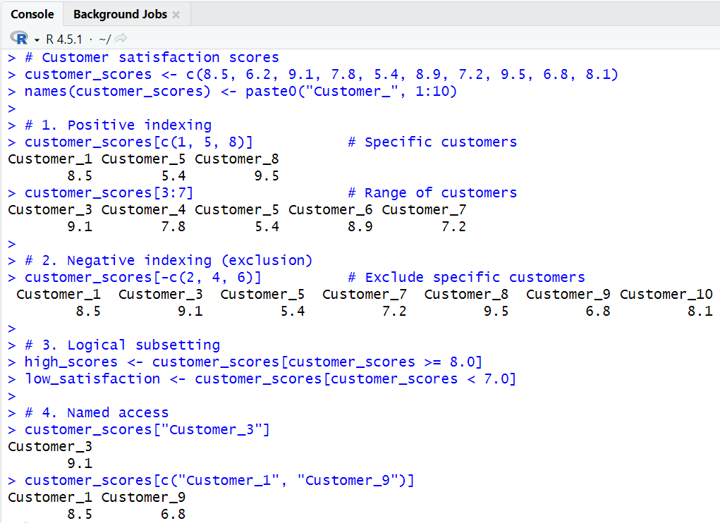
# Customer satisfaction scores
customer_scores <- c(8.5, 6.2, 9.1, 7.8, 5.4, 8.9, 7.2, 9.5, 6.8, 8.1)
names(customer_scores) <- paste0("Customer_", 1:10)

# 1. Positive indexing
customer_scores[c(1, 5, 8)]           # Specific customers
customer_scores[3:7]                  # Range of customers

# 2. Negative indexing (exclusion)
customer_scores[-c(2, 4, 6)]          # Exclude specific customers

# 3. Logical subsetting
high_scores <- customer_scores[customer_scores >= 8.0]
low_satisfaction <- customer_scores[customer_scores < 7.0]

# 4. Named access
customer_scores["Customer_3"]
customer_scores[c("Customer_1", "Customer_9")]
- Explanation:
customer_scores[c(1, 5, 8)]- Selects the 1st, 5th, and 8th elements from the vector, returning the scores for these specific customers.
customer_scores[3:7]- Selects a range of elements from the 3rd to the 7th, returning the scores for these customers.
customer_scores[-c(2, 4, 6)]- Excludes the 2nd, 4th, and 6th customers, returning scores for all other customers.
high_scores <- customer_scores[customer_scores >= 8.0]- Creates a new vector with scores that are 8.0 or higher.
low_satisfaction <- customer_scores[customer_scores < 7.0]- Creates a new vector with scores lower than 7.0.
customer_scores["Customer_3"]- Selects the element named "Customer_3", returning the score for this customer.
customer_scores[c("Customer_1", "Customer_9")]- Selects multiple elements by their names, returning the scores for these customers.
Data Frame Subsetting
- Accessing Rows and Columns:
- Data frames can be subset by row and column indices, names, or logical conditions.
# Employee dataset
employee_data <- data.frame(
  Name = c("Sarah", "Mike", "Lisa", "Tom", "Ana"),
  Department = c("Sales", "IT", "HR", "Sales", "IT"),
  Salary = c(55000, 62000, 58000, 51000, 65000),
  Years_Experience = c(3, 5, 7, 2, 6)
)

# Row and column access
employee_data[2, ]                    # Mike's data
employee_data[, "Salary"]             # All salaries
employee_data[1:3, c("Name", "Department")]  # First 3 employees

# Conditional subsetting
sales_team <- employee_data[employee_data$Department == "Sales", ]
senior_staff <- employee_data[employee_data$Years_Experience >= 5, ]
high_earners <- employee_data[employee_data$Salary > 60000, c("Name", "Salary")]
- Explanation:
employee_datais a data frame with columns for employee name, department, salary, and years of experience.employee_data[2, ]- Selects the entire second row, returning all information for "Mike".
employee_data[, "Salary"]- Selects the "Salary" column for all employees, returning a vector of salaries.
employee_data[1:3, c("Name", "Department")]- Selects the first three rows and only the "Name" and "Department" columns, returning a smaller data frame.
sales_team <- employee_data[employee_data$Department == "Sales", ]- Filters the data frame to include only employees in the "Sales" department.
senior_staff <- employee_data[employee_data$Years_Experience >= 5, ]- Filters for employees with five or more years of experience.
high_earners <- employee_data[employee_data$Salary > 60000, c("Name", "Salary")]- Selects only the names and salaries of employees earning more than 60,000.
4. R Data Types: Basic Types
- Atomic Types:
- R's atomic types are the building blocks for all other structures: logical, integer, numeric, complex, character, and raw.
4.1 Logical
- TRUE/FALSE Values:
- Used for flags, conditions, and logical operations.
# Quality control flags
passed_inspection <- c(TRUE, TRUE, FALSE, TRUE, FALSE, TRUE)
is_premium <- c(FALSE, TRUE, FALSE, FALSE, TRUE, TRUE)

# Logical operations
all_passed <- all(passed_inspection)          # FALSE
any_premium <- any(is_premium)                # TRUE
premium_count <- sum(is_premium)              # 3 (TRUE counts as 1)

# Combining conditions
premium_and_passed <- is_premium & passed_inspection
premium_or_passed <- is_premium | passed_inspection
- Explanation:
- Shows how to combine logical vectors and count TRUE values.
**Common Warning Scenarios**
Mixing logical and numeric types
x <- c(TRUE, 1, FALSE)- R coerces logicals to numeric (TRUE = 1, FALSE = 0) silently.
Logical operations on non-logical data
y <- c("yes", "no", "maybe") z <- y & TRUE- Warning: NAs introduced by coercion.
**Typical Error Triggers**
Invalid logical comparisons
x <- c(TRUE, FALSE) x > 1- Returns FALSE, but may not be meaningful.
Length mismatch in logical indexing
x <- c(TRUE, FALSE) y <- 1:3 y[x]- Warning: longer object length is not a multiple of shorter object length.
4.2 Integer
- Whole Numbers:
- Use less memory than numeric (double) types.
# Inventory counts (integers save memory for whole numbers)
widget_inventory <- as.integer(c(150, 89, 234, 67, 445))
batch_numbers <- 1001L:1050L  # L suffix ensures integer type

class(widget_inventory)       # "integer"
is.integer(batch_numbers)     # TRUE
storage.mode(widget_inventory) # "integer" (more memory efficient)
- Explanation:
- Demonstrates integer creation and checking type.
**Common Warning Scenarios**
Mixing integer and numeric
x <- c(1L, 2.5)- Coerces to numeric (double).
Large integer values
x <- 2^31- Stored as numeric, not integer.
**Typical Error Triggers**
Assigning non-integer to integer vector
x <- integer(2) x[1] <- 3.5- Value truncated to 3.
Overflow
x <- as.integer(2^31)- Results in NA with warning: NAs introduced by coercion.
4.3 Numeric (Double)
- Decimal Numbers:
- Used for precise calculations.
# Financial calculations requiring precision
stock_prices <- c(134.56, 89.23, 156.78, 201.45, 78.90)
price_changes <- c(-2.34, +5.67, -0.89, +12.45, -3.21)
percentage_change <- price_changes / stock_prices * 100

# Mathematical operations
volatility <- sd(price_changes)                    # Standard deviation
moving_average <- mean(stock_prices[1:3])          # First 3 stocks
- Explanation:
- Shows financial calculations and statistical summaries.
**Common Warning Scenarios**
Precision loss
x <- 0.1 + 0.2 x == 0.3- Returns FALSE due to floating-point precision.
Mixing numeric and character
x <- c(1.5, "two")- Coerces to character.
**Typical Error Triggers**
- Non-numeric input to numeric functions
mean("apple")- Error: argument is not numeric or logical: returning NA.
4.4 Complex
- Complex Numbers:
- Useful in engineering and scientific calculations.
# Engineering calculations with complex numbers
impedance_values <- c(3+4i, 2-5i, 1+1i, 4+0i)
phase_angles <- Arg(impedance_values)              # Phase angles
magnitudes <- Mod(impedance_values)               # Magnitudes

# Complex arithmetic
total_impedance <- sum(impedance_values)
power_factor <- Re(impedance_values) / Mod(impedance_values)
- Explanation:
- Demonstrates operations on complex numbers, such as magnitude and phase.
**Common Warning Scenarios**
Mixing complex and real
x <- c(1+2i, 3)- 3 is coerced to 3+0i.
Coercion to complex
as.complex("abc")- Warning: NAs introduced by coercion.
**Typical Error Triggers**
- Invalid operations
sqrt(-1)- Returns NaN unless explicitly using complex numbers.
4.5 Character
- Text Data:
- Used for names, labels, and string manipulation.
# Customer database
customer_names <- c("Johnson Electronics", "Smith & Co", "Brown Industries")
email_addresses <- c("info@johnson.com", "contact@smith.co", "sales@brown.ind")

# String operations
name_lengths <- nchar(customer_names)             # Character counts
total_contacts <- length(customer_names)          # Number of customers

# String manipulation
full_contact <- paste(customer_names, email_addresses, sep = " - ")
company_codes <- substr(customer_names, 1, 3)    # First 3 characters
uppercase_names <- toupper(customer_names)
- Explanation:
- Shows string operations like counting characters, concatenation, and case conversion.
**Common Warning Scenarios**
Mixing character and numeric
x <- c("a", 1)- Coerces all to character.
NA in character operations
x <- c("a", NA) nchar(x)- Returns NA for missing values.
**Typical Error Triggers**
Invalid substring indices
substr("abc", 2, 1)- Returns "" (empty string).
Non-character input to string functions
nchar(123)- Works (coerces to character), but may be unexpected.
4.6 Raw
- Binary Data:
- Used for low-level data storage and manipulation.
# Binary data handling
file_header <- charToRaw("PNG")                   # Convert to raw bytes
hex_values <- as.raw(c(137, 80, 78, 71))         # PNG file signature
binary_data <- as.raw(0:255)                     # Full byte range
- Explanation:
- Demonstrates conversion to raw bytes and handling binary data.
**Common Warning Scenarios**
Coercion to raw
as.raw(300)- Warning: out-of-range values are truncated modulo 256.
Mixing raw and other types
x <- c(as.raw(1), 2)- Coerces to integer.
**Typical Error Triggers**
- Invalid conversion
as.raw("abc")- Error: cannot coerce type 'character' to vector of type 'raw'.
5. R Data Types: Vector
- Homogeneous Sequences:
- Vectors are the backbone of R, storing data of a single type.
Vector Characteristics and Operations
- Properties and Naming:
- Vectors can be named for easier access and summarized with functions like
length()andsum().
- Vectors can be named for easier access and summarized with functions like
# Product catalog
product_names <- c("Laptop", "Mouse", "Keyboard", "Monitor", "Webcam")
product_prices <- c(899.99, 25.50, 89.00, 299.99, 75.00)

# Vector properties
length(product_names)                 # 5
sum(nchar(product_names))            # Total characters: 28

# Named vectors (dictionary-style)
names(product_prices) <- product_names
product_prices["Laptop"]             # 899.99
product_prices[c("Mouse", "Webcam")] # Multiple items
- Explanation:
- Shows how to name vector elements and access them by name.
Vector Combination and Recycling
- Combining and Recycling:
- Vectors can be combined, and shorter vectors are recycled in operations.
electronics <- c("Smartphone", "Tablet", "Headphones")
accessories <- c("Case", "Charger", "Stand", "Cable")

# Combine vectors
all_products <- c(electronics, accessories)
# Result: "Smartphone", "Tablet", "Headphones", "Case", "Charger", "Stand", "Cable"

# Element-wise string operations
category_prefix <- c("ELEC", "ACC")
product_codes <- paste(category_prefix, 1:7, sep="-")
# Recycling: "ELEC-1", "ACC-2", "ELEC-3", "ACC-4", "ELEC-5", "ACC-6", "ELEC-7"
- Explanation:
- Demonstrates combining vectors and recycling in string operations.
6. R Data Types: List
- Heterogeneous Containers:
- Lists can hold any type of R object, including other lists.
Basic List Creation and Access
- Creating Lists:
- Lists can contain vectors, data frames, and other objects.
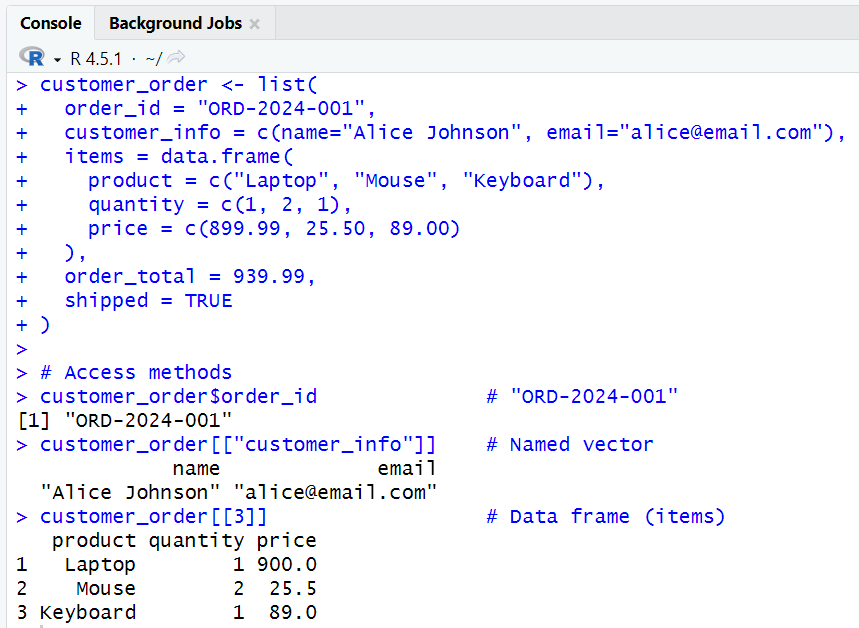
# Customer order information
customer_order <- list(
  order_id = "ORD-2024-001",
  customer_info = c(name="Alice Johnson", email="alice@email.com"),
  items = data.frame(
    product = c("Laptop", "Mouse", "Keyboard"),
    quantity = c(1, 2, 1),
    price = c(899.99, 25.50, 89.00)
  ),
  order_total = 939.99,
  shipped = TRUE
)

# Access methods
customer_order$order_id              # "ORD-2024-001"
customer_order[["customer_info"]]    # Named vector
customer_order[[3]]                  # Data frame (items)
Output:
- Explanation:
customer_orderis a list containing various elements: a character string for the order ID, a named vector for customer info, a data frame for items, a numeric value for order total, and a logical value for shipment status.customer_order$order_id- Extracts the
order_idelement from the list.
- Extracts the
customer_order[["customer_info"]]- Extracts the
customer_infoelement as a named vector.
- Extracts the
customer_order[[3]]- Extracts the third element (data frame of items) from the list.
**Nested Lists**
- Lists within Lists:
- Useful for representing hierarchical or grouped data.
# Sales reporting system
quarterly_report <- list(
  Q1 = list(
    revenue = c(Jan=45000, Feb=52000, Mar=48000),
    top_products = c("Widget A", "Widget B", "Widget C"),
    customer_count = 234
  ),
  Q2 = list(
    revenue = c(Apr=55000, May=61000, Jun=58000),
    top_products = c("Widget B", "Widget D", "Widget A"),
    customer_count = 267
  )
)

**Nested access**
quarterly_report$Q1$revenue["Feb"]   # 52000
quarterly_report[[1]][[1]][2]        # 52000 (same result)
quarterly_report$Q2$customer_count   # 267
- Explanation:
quarterly_reportis a nested list: each quarter (Q1, Q2) contains its own list with elements for revenue, top products, and customer count.quarterly_report$Q1$revenue["Feb"]- Accesses the revenue for February in Q1.
quarterly_report[[1]][[1]][2]- Another way to access the same value using double bracket notation.
quarterly_report$Q2$customer_count- Accesses the customer count for Q2.
**List Manipulation**
- Modifying Lists:
- Lists can be expanded or processed with functions like
sapply().
- Lists can be expanded or processed with functions like
# Add new quarter
quarterly_report$Q3 <- list(
  revenue = c(Jul=63000, Aug=59000, Sep=65000),
  top_products = c("Widget D", "Widget A", "Widget E"),
  customer_count = 289
)

# Extract all customer counts
customer_counts <- sapply(quarterly_report, function(q) q$customer_count)
# Result: Q1=234, Q2=267, Q3=289
- Explanation:
quarterly_report$Q3 <- list(...)- Adds a new element for Q3 with its own nested list.
sapply(quarterly_report, function(q) q$customer_count)- Applies a function to each element of the
quarterly_reportlist, extracting thecustomer_countfrom each sub-list.
- Applies a function to each element of the
7. R Data Types: Factor
- Categorical Data:
- Factors efficiently store categorical variables with fixed levels.
Creating and Managing Factors
- Defining Levels:
- Factors can be ordered or unordered, and levels can be set explicitly.
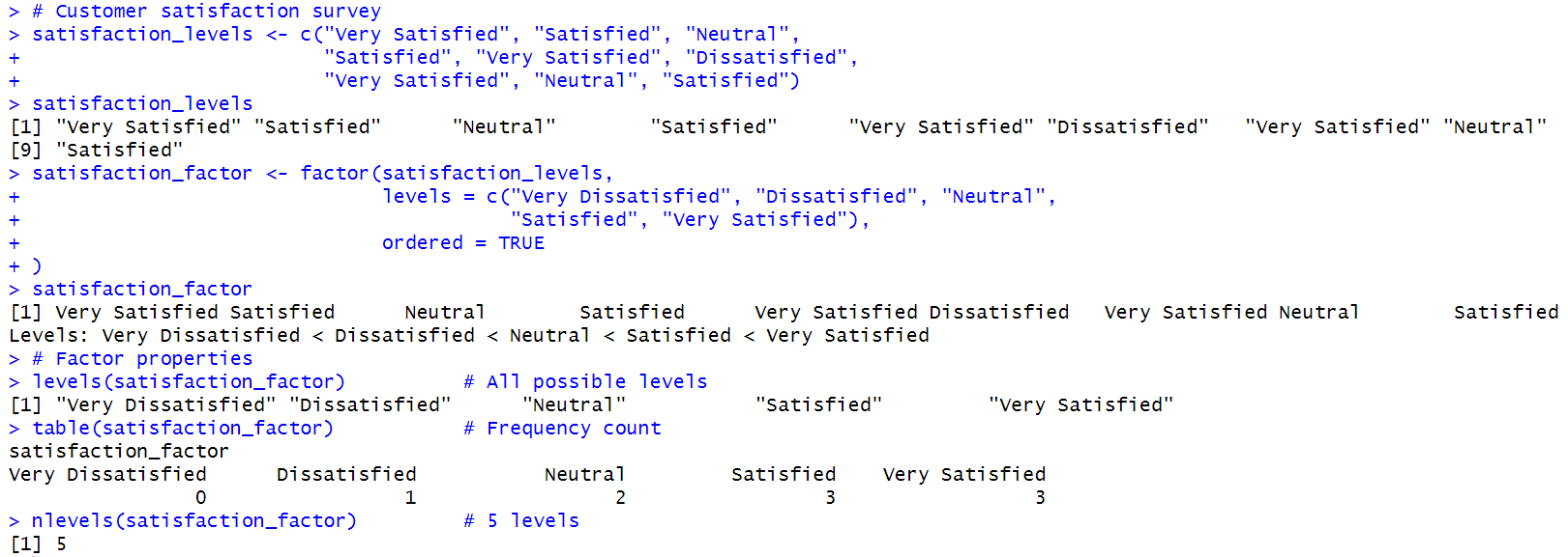
# Customer satisfaction survey
satisfaction_levels <- c("Very Satisfied", "Satisfied", "Neutral",
                        "Satisfied", "Very Satisfied", "Dissatisfied",
                        "Very Satisfied", "Neutral", "Satisfied")

satisfaction_factor <- factor(satisfaction_levels,
  levels = c("Very Dissatisfied", "Dissatisfied", "Neutral",
             "Satisfied", "Very Satisfied"),
  ordered = TRUE
)

# Factor properties
levels(satisfaction_factor)          # All possible levels
table(satisfaction_factor)           # Frequency count
nlevels(satisfaction_factor)         # 5 levels
Output:
- Explanation:
satisfaction_levelsis a character vector of survey responses.factor(satisfaction_levels, levels = ..., ordered = TRUE)- Converts the character vector to an ordered factor, specifying the order of levels.
levels(satisfaction_factor)- Returns the defined levels of the factor.
table(satisfaction_factor)- Provides a frequency count of each level in the factor.
nlevels(satisfaction_factor)- Returns the number of levels in the factor.
Factor Operations
- Analyzing and Modifying Factors:
- Frequency tables and level modification are common operations.
# Product categories
product_categories <- factor(c("Electronics", "Clothing", "Books",
                              "Electronics", "Home", "Books", "Clothing"),
                            levels = c("Electronics", "Clothing", "Books", "Home", "Sports"))

# Frequency analysis
category_counts <- table(product_categories)
# Electronics: 2, Clothing: 2, Books: 2, Home: 1, Sports: 0

# Level modification
levels(product_categories)[levels(product_categories) == "Electronics"] <- "Tech"
# Changes "Electronics" to "Tech" throughout the factor
- Explanation:
product_categoriesis a factor representing the category of each product.table(product_categories)- Creates a frequency table showing the count of each category.
levels(product_categories)[levels(product_categories) == "Electronics"] <- "Tech"- Modifies the levels of the factor, renaming "Electronics" to "Tech".
Ordered Factors
- Ordered Categories:
- Useful for ordinal data where order matters.
# Priority levels
task_priority <- ordered(c("High", "Medium", "Low", "High", "Medium"),
                        levels = c("Low", "Medium", "High"))

# Ordered comparisons
high_priority_tasks <- task_priority >= "Medium"  # TRUE, TRUE, FALSE, TRUE, TRUE
urgent_count <- sum(task_priority == "High")      # 2
- Explanation:
task_priorityis an ordered factor representing the priority of tasks.task_priority >= "Medium"- Compares each element to "Medium", returning a logical vector indicating if the condition is TRUE or FALSE for each task.
sum(task_priority == "High")- Counts the number of tasks with "High" priority.
8. R Data Types: Matrix
- 2D Homogeneous Storage:
- Matrices store data of a single type in two dimensions.
Matrix Creation and Properties
- Creating Matrices:
- Use
matrix()and set row/column names for clarity.
- Use
# Sales data by month and region
sales_matrix <- matrix(
  c(15000, 18000, 22000, 19000,    # Region 1
    12000, 16000, 20000, 17000,    # Region 2
    14000, 15000, 18000, 16000),   # Region 3
  nrow = 3, ncol = 4, byrow = TRUE,
  dimnames = list(
    Region = c("North", "South", "West"),
    Month = c("Jan", "Feb", "Mar", "Apr")
  )
)

dim(sales_matrix)                    # 3 4 (3 rows, 4 columns)
rownames(sales_matrix)               # "North", "South", "West"
colnames(sales_matrix)               # "Jan", "Feb", "Mar", "Apr"
Output:

- Explanation:
sales_matrixis a matrix with 3 rows and 4 columns, filled by rows with sales data for three regions over four months.dim(sales_matrix)- Returns the dimensions of the matrix: 3 rows and 4 columns.
rownames(sales_matrix)andcolnames(sales_matrix)- Return the row and column names, respectively.
Matrix Operations
- Mathematical Operations:
- Row/column sums, element-wise arithmetic, and transposition.
# Mathematical operations
total_by_region <- rowSums(sales_matrix)    # Regional totals
total_by_month <- colSums(sales_matrix)     # Monthly totals
overall_total <- sum(sales_matrix)          # Grand total

# Matrix arithmetic
growth_factors <- matrix(c(1.05, 1.08, 1.12, 1.10), nrow = 3, ncol = 4, byrow = TRUE)
projected_sales <- sales_matrix * growth_factors  # Element-wise multiplication

# Matrix transpose
monthly_by_region <- t(sales_matrix)        # 4x3 matrix (months as rows)
- Explanation:
rowSums(sales_matrix)andcolSums(sales_matrix)- Calculate the sum of each row and each column, respectively.
sum(sales_matrix)- Calculates the grand total of all elements in the matrix.
t(sales_matrix)- Transposes the matrix, swapping rows and columns.
Matrix Subsetting
- Extracting Data:
- Access elements by row/column names or indices.
# Access specific elements
sales_matrix["North", "Mar"]         # North region, March sales
sales_matrix[1, ]                    # First row (North region)
sales_matrix[, "Feb"]                # February column
sales_matrix[c("North", "South"), c("Jan", "Mar")]  # Subset regions and months
- Explanation:
sales_matrix["North", "Mar"]- Selects the element at the intersection of the "North" row and "Mar" column.
sales_matrix[1, ]- Selects the entire first row, returning all data for the "North" region.
sales_matrix[, "Feb"]- Selects the entire "Feb" column, returning sales data for February across all regions.
sales_matrix[c("North", "South"), c("Jan", "Mar")]- Selects specific rows and columns, returning a subset of the matrix.
**Common Warning Scenarios**
Mixing types in matrix
m <- matrix(c(1, "a"), nrow=1)- All elements coerced to character.
Assigning wrong length
m <- matrix(1:4, 2, 2) m[] <- 1:3- Warning: number of items to replace is not a multiple of replacement length.
**Typical Error Triggers**
Invalid subscript
m <- matrix(1:4, 2, 2) m[3, 1]- Error: subscript out of bounds.
Assigning incompatible type
m <- matrix(1:4, 2, 2) m[1,1] <- list(1)- Error: replacement has length zero.
9. R Data Types: Array
- Multi-dimensional Data:
- Arrays generalize matrices to more than two dimensions.
Creating Multi-dimensional Arrays
- Defining Dimensions:
- Use
array()and specify dimension names for clarity.
- Use
# Sales data by Product × Region × Quarter
sales_array <- array(
  data = c(
    # Product A: Regions × Quarters
    15000, 12000, 14000,  # Q1: North, South, West
    18000, 16000, 15000,  # Q2: North, South, West
    # Product B: Regions × Quarters
    22000, 20000, 18000,  # Q1: North, South, West
    25000, 23000, 21000   # Q2: North, South, West
  ),
  dim = c(3, 2, 2),  # 3 regions, 2 quarters, 2 products
  dimnames = list(
    Region = c("North", "South", "West"),
    Quarter = c("Q1", "Q2"),
    Product = c("Product_A", "Product_B")
  )
)
- Explanation:
sales_arrayis a 3-dimensional array with dimensions for regions, quarters, and products, containing sales data for two products across two quarters in three regions.dim(sales_array)- Returns the dimensions of the array: 3 regions, 2 quarters, and 2 products.
dimnames(sales_array)- Sets the names for each dimension, allowing for easier identification of data.
Array Access and Operations
- Accessing and Summarizing:
- Use indices and
apply()to extract and summarize data along dimensions.
- Use indices and
# Access specific elements
sales_array["North", "Q2", "Product_B"]     # 25000
sales_array[, "Q1", ]                       # All regions, Q1, all products
sales_array["South", , "Product_A"]         # South region, all quarters, Product A

# Calculations across dimensions
regional_totals <- apply(sales_array, 1, sum)      # Sum by region
quarterly_totals <- apply(sales_array, 2, sum)     # Sum by quarter
product_totals <- apply(sales_array, 3, sum)       # Sum by product
- Explanation:
sales_array["North", "Q2", "Product_B"]- Selects the sales figure for Product B in the North region for Q2.
apply(sales_array, 1, sum)- Applies the
sumfunction across the first dimension (rows), calculating total sales for each region.
- Applies the
apply(sales_array, 2, sum)- Applies the
sumfunction across the second dimension (columns), calculating total sales for each quarter.
- Applies the
apply(sales_array, 3, sum)- Applies the
sumfunction across the third dimension (slices), calculating total sales for each product.
- Applies the
Array Manipulation
- Expanding Arrays:
- Arrays can be extended by combining with new data (using packages like
abind).
- Arrays can be extended by combining with new data (using packages like
# Add new quarter data
Q3_data <- array(c(20000, 18000, 16000, 28000, 26000, 24000),
                dim = c(3, 1, 2),
                dimnames = list(c("North", "South", "West"), "Q3", c("Product_A", "Product_B")))

# Combine arrays (would require abind package in practice)
# expanded_sales <- abind(sales_array, Q3_data, along = 2)
- Explanation:
Q3_datais a new array containing sales data for Q3, structured similarly to the originalsales_array.abind(sales_array, Q3_data, along = 2)- This hypothetical line (commented out) would combine the original sales array with the new Q3 data along the second dimension (quarters), expanding the array to include the new data.
10. R Data Types: Data Frame
- Spreadsheet-like Tables:
- Data frames store heterogeneous columns, similar to Excel tables.
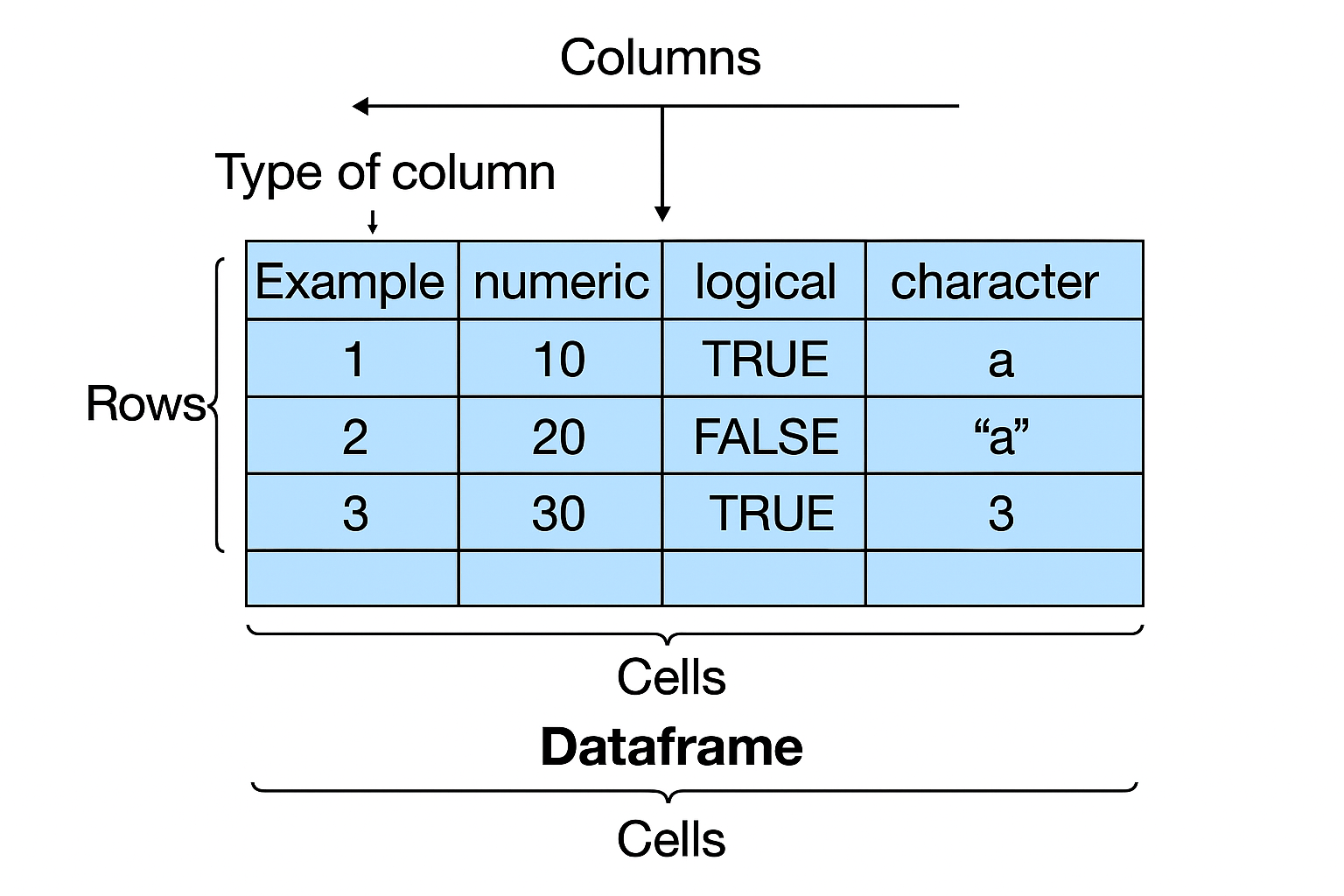
Creating and Managing Data Frames
- Defining Data Frames:
- Use
data.frame()to create tables with named columns of different types.
- Use
# Employee management system
employee_df <- data.frame(
  EmployeeID = c(1001, 1002, 1003, 1004, 1005),
  Name = c("Sarah Wilson", "Mike Chen", "Lisa Anderson", "Tom Rodriguez", "Ana Petrov"),
  Department = factor(c("Sales", "Engineering", "HR", "Sales", "Engineering")),
  Salary = c(65000, 85000, 58000, 62000, 90000),
  StartDate = as.Date(c("2020-03-15", "2019-07-22", "2021-01-10", "2020-11-05", "2018-09-30")),
  Remote = c(FALSE, TRUE, FALSE, TRUE, TRUE),
  stringsAsFactors = FALSE
)

# Data frame properties
str(employee_df)                     # Structure overview
nrow(employee_df)                    # 5 employees
ncol(employee_df)                    # 6 columns
names(employee_df)                   # Column names
- Explanation:
employee_dfis a data frame with columns for employee ID, name, department, salary, start date, and remote work status.str(employee_df)- Displays the structure of the data frame, including the type and example values of each column.
nrow(employee_df)andncol(employee_df)- Return the number of rows (employees) and columns (attributes) in the data frame, respectively.
names(employee_df)- Returns the names of the columns in the data frame.
Data Frame Operations
- Accessing and Filtering:
- Access columns by name, filter rows by condition, and add new columns.
# Column access
employee_df$Name                     # Name column
employee_df[["Salary"]]             # Salary column
employee_df$Department              # Factor column

# Row filtering
engineering_team <- employee_df[employee_df$Department == "Engineering", ]
high_earners <- employee_df[employee_df$Salary >= 70000, ]
remote_workers <- employee_df[employee_df$Remote == TRUE, c("Name", "Department")]

# Adding new data
employee_df$YearsService <- as.numeric(Sys.Date() - employee_df$StartDate) / 365.25
employee_df$SalaryGrade <- cut(employee_df$Salary,
                              breaks = c(0, 60000, 80000, Inf),
                              labels = c("Junior", "Mid", "Senior"))
- Explanation:
employee_df$Name- Extracts the "Name" column as a character vector.
employee_df[["Salary"]]- Extracts the "Salary" column as a numeric vector.
employee_df$Department- Extracts the "Department" column, which is a factor (categorical variable).
engineering_team <- employee_df[employee_df$Department == "Engineering", ]- Filters the data frame to include only employees in the "Engineering" department.
high_earners <- employee_df[employee_df$Salary >= 70000, ]- Filters for employees with a salary of 70,000 or more.
remote_workers <- employee_df[employee_df$Remote == TRUE, c("Name", "Department")]- Selects the names and departments of employees who work remotely.
employee_df$YearsService <- as.numeric(Sys.Date() - employee_df$StartDate) / 365.25- Calculates the number of years each employee has worked by subtracting their start date from the current date and dividing by 365.25 (to account for leap years).
- Adds this as a new column "YearsService".
employee_df$SalaryGrade <- cut(employee_df$Salary, breaks = c(0, 60000, 80000, Inf), labels = c("Junior", "Mid", "Senior"))- Categorizes employees into "Junior", "Mid", or "Senior" based on their salary, and adds this as a new column.
Data Frame Summary and Analysis
- Summarizing Data:
- Use
summary(),mean(),table(), andaggregate()for quick analysis.
- Use
# Statistical summaries
summary(employee_df)                 # Overall summary
mean(employee_df$Salary)             # Average salary: 72000
table(employee_df$Department)        # Department distribution

# Advanced operations
by_dept_salary <- aggregate(Salary ~ Department, employee_df, mean)
# Average salary by department
- Explanation:
summary(employee_df)- Provides a summary of each column in the data frame, including min, max, mean, and quartiles for numeric columns, and counts for factors.
mean(employee_df$Salary)- Calculates the average salary across all employees.
table(employee_df$Department)- Counts the number of employees in each department.
by_dept_salary <- aggregate(Salary ~ Department, employee_df, mean)- Groups the data by department and calculates the mean salary for each group, returning a summary table.
11. Data Frames: Order and Merge
- Sorting and Joining:
- Data frames can be sorted by one or more columns and merged (joined) with others.
Ordering Data Frames
- Sorting Rows:
- Use
order()to sort by one or more columns.
- Use
# Customer transaction data
transaction_df <- data.frame(
  CustomerID = c(101, 102, 101, 103, 102, 104),
  TransactionDate = as.Date(c("2024-01-15", "2024-01-18", "2024-01-20",
                             "2024-01-22", "2024-01-25", "2024-01-28")),
  Amount = c(150.00, 89.50, 220.00, 175.50, 95.00, 310.00),
  Product = c("Widget A", "Widget B", "Widget C", "Widget A", "Widget B", "Widget D")
)

# Single column sorting
by_amount <- transaction_df[order(transaction_df$Amount), ]              # Ascending
by_amount_desc <- transaction_df[order(transaction_df$Amount, decreasing = TRUE), ] # Descending

# Multiple column sorting
by_customer_date <- transaction_df[order(transaction_df$CustomerID, transaction_df$TransactionDate), ]
by_customer_amount <- transaction_df[order(transaction_df$CustomerID, -transaction_df$Amount), ]
- Explanation:
transaction_dfis a data frame containing transaction data with columns for customer ID, transaction date, amount, and product.order(transaction_df$Amount)- Returns the order of indices that would sort the
Amountcolumn in ascending order.
- Returns the order of indices that would sort the
transaction_df[order(transaction_df$Amount), ]- Reorders the rows of the data frame according to the sorted order of the
Amountcolumn, giving a data frame sorted by transaction amount.
- Reorders the rows of the data frame according to the sorted order of the
transaction_df[order(transaction_df$Amount, decreasing = TRUE), ]- Sorts the data frame by transaction amount in descending order.
order(transaction_df$CustomerID, transaction_df$TransactionDate)- Returns the order of indices that would sort the data first by
CustomerIDand then byTransactionDatewithin each customer ID group.
- Returns the order of indices that would sort the data first by
transaction_df[order(transaction_df$CustomerID, transaction_df$TransactionDate), ]- Sorts the data frame first by customer ID and then by transaction date.
Data Frame Merging
- Combining Data Frames:
- Use
merge()for inner, left, and full joins.
- Use
# Customer information
customer_info <- data.frame(
  CustomerID = c(101, 102, 103, 104, 105),
  CustomerName = c("ABC Corp", "XYZ Ltd", "Johnson Inc", "Smith Co", "Brown LLC"),
  CustomerType = c("Premium", "Standard", "Premium", "Standard", "Premium")
)

# Transaction summary
transaction_summary <- data.frame(
  CustomerID = c(101, 102, 103, 104),
  TotalAmount = c(370.00, 184.50, 175.50, 310.00),
  TransactionCount = c(2, 2, 1, 1)
)

# Different join types
# Inner join (only matching records)
inner_result <- merge(customer_info, transaction_summary, by = "CustomerID")

# Left join (all customers, matched transactions)
left_result <- merge(customer_info, transaction_summary, by = "CustomerID", all.x = TRUE)

# Full outer join (all records from both)
full_result <- merge(customer_info, transaction_summary, by = "CustomerID", all = TRUE)

# Add merge indicator
full_result$merge_flag <- with(full_result,
  ifelse(!is.na(CustomerName) & is.na(TotalAmount), "customer_only",
         ifelse(is.na(CustomerName) & !is.na(TotalAmount), "transaction_only", "both")))
- Explanation:
customer_infoandtransaction_summaryare data frames containing customer details and transaction summaries, respectively.merge(customer_info, transaction_summary, by = "CustomerID")- Performs an inner join, merging the two data frames by
CustomerIDand keeping only the rows with matchingCustomerIDin both data frames.
- Performs an inner join, merging the two data frames by
merge(customer_info, transaction_summary, by = "CustomerID", all.x = TRUE)- Performs a left join, keeping all rows from
customer_infoand adding matching rows fromtransaction_summary. - If there is no match,
NAis filled in for columns fromtransaction_summary.
- Performs a left join, keeping all rows from
merge(customer_info, transaction_summary, by = "CustomerID", all = TRUE)- Performs a full outer join, keeping all rows from both data frames and filling in
NAwhere there are no matches.
- Performs a full outer join, keeping all rows from both data frames and filling in
full_result$merge_flag <- with(full_result, ...)- Creates a new column
merge_flagto indicate the source of each row: "customer_only", "transaction_only", or "both".
- Creates a new column
Advanced Merging Examples
- Merging on Multiple Keys:
- Useful for combining detailed transaction and product data.
# Multiple key merging
product_sales <- data.frame(
  Product = c("Widget A", "Widget B", "Widget C", "Widget D"),
  Category = c("Electronics", "Electronics", "Home", "Home"),
  UnitPrice = c(25.00, 15.50, 45.00, 65.00)
)

detailed_transactions <- merge(
  transaction_df,
  product_sales,
  by = "Product",
  all.x = TRUE
)

# Calculate extended amounts
detailed_transactions$ExtendedAmount <-
  detailed_transactions$Amount / detailed_transactions$UnitPrice * detailed_transactions$UnitPrice
- Explanation:
product_salesis a data frame containing product details, including unit price.merge(transaction_df, product_sales, by = "Product", all.x = TRUE)- Merges transaction data with product details by
Product, adding product information to each transaction.
- Merges transaction data with product details by
detailed_transactions$ExtendedAmount <- ...- Calculates the extended amount for each transaction based on the unit price and amount.
Performance & Memory Optimization
- Tips for Efficient R Code:
- Pre-allocate vectors for loops to avoid memory overhead.
- Use vectorized operations for speed.
- Store categorical data as factors to save memory.
- Use matrices for fast linear algebra.
- For large data, use
data.tablefor performance.
Quick Reference Summary
| Structure | Creation Function | Access Method | Key Benefit |
|---|---|---|---|
| Vector | c(), seq() |
vec[i], vec["name"] |
Vectorized operations |
| Factor | factor(), ordered() |
fac[i], levels() |
Categorical efficiency |
| Matrix | matrix(), cbind() |
mat[i,j] |
Mathematical operations |
| Array | array() |
arr[i,j,k,...] |
Multi-dimensional data |
| Data Frame | data.frame() |
df$col, df[i,j] |
Mixed-type datasets |
| List | list() |
list[[i]], list$name |
Flexible containers |
**Resource download links**
1.2.2.-Data-Structures-or-Objects-in-R.zip