2.1.1. Introduction to Tidy Data (Tidyverse)
1. Introduction to Tidy Data and Its Terminology
Tidy data is a foundational concept in data science, especially in R. Understanding tidy data principles makes data analysis, visualization, and modeling much easier and more reliable.
What is Tidy Data?
Tidy data is a standardized way of organizing datasets to facilitate analysis. The core idea is that each variable forms a column, each observation forms a row, and each type of observational unit forms a table.
Key Principles of Tidy Data
- Each variable forms a column
- Each observation forms a row
- Each type of observational unit forms a table
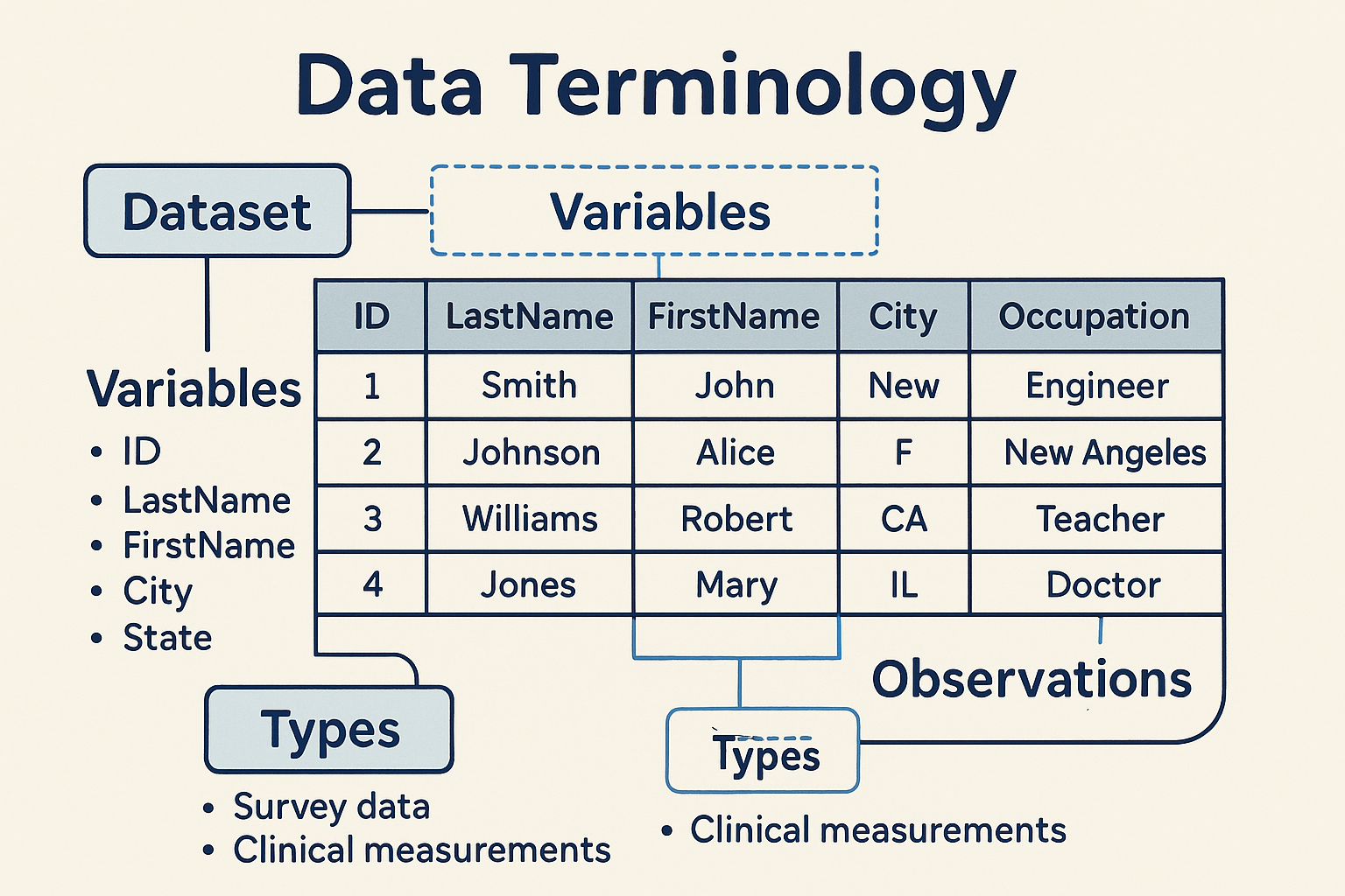
**Data Terminology**
Before diving deeper, let's clarify some essential terms:
Dataset
- A dataset is a collection of values, typically organized in a table or spreadsheet.
- Every value in a dataset belongs to a variable and an observation.
Variables
- Variables are the different categories or attributes measured in the dataset.
- Each variable is represented as a column.
- Example variables:
ID,LastName,FirstName,Sex,City,State,Occupation.
Observations
- An observation is a single measurement or record, typically represented as a row.
- Each observation contains values for every variable.
Types
- Sometimes, data about the same individuals comes from multiple sources or types.
- Example: Survey data vs. clinical measurements.
**What is Untidy Data?**
Untidy data (or messy data) refers to datasets that do not follow the tidy data principles. Common characteristics of untidy data include:
- Variables spread across multiple columns or rows
- Multiple types of data mixed in a single table
- Blank cells or missing values not handled consistently
- Data not arranged in a rectangular format (i.e., not every row has the same columns)
- Repeated information or inconsistent variable names
Untidy data makes analysis, visualization, and data manipulation more difficult and error-prone.

**Tidying Untidy Data**
There are several actions you can take to tidy a dataset, depending on the specific issues present. These include:
- Filtering: Removing unnecessary rows or columns.
- Transforming: Changing the structure of the data (e.g., pivoting from wide to long format).
- Modifying Variables: Renaming columns, changing data types, or creating new variables.
- Aggregating: Summarizing data by groups or categories.
- Sorting: Arranging observations in a specific order.
R provides functions for each of these actions. While the details of the code will be covered in later lessons, it is important to first recognize untidy data and determine what steps are needed to tidy it.
**Example: Tidy Data Structure**
Clinical data is often collected in a way that is not tidy, especially in raw data exports. Below is an example using SDTM-like domains (Demographics and Adverse Events).
Input Table (Untidy Clinical Data Example)
| USUBJID | AGE | SEX | AE1TERM | AE1SEV | AE2TERM | AE2SEV |
|---|---|---|---|---|---|---|
| ABC123-01 | 45 | M | Headache | MILD | Nausea | MODERATE |
| ABC123-02 | 52 | F | Dizziness | SEVERE |
- Here, adverse events are stored in separate columns (AE1TERM, AE2TERM, etc.), which is not tidy.
Tidy Output Table (Clinical Data)
| USUBJID | AGE | SEX | AESEQ | AETERM | AESEV |
|---|---|---|---|---|---|
| ABC123-01 | 45 | M | 1 | Headache | MILD |
| ABC123-01 | 45 | M | 2 | Nausea | MODERATE |
| ABC123-02 | 52 | F | 1 | Dizziness | SEVERE |
- Now, each adverse event is a separate row, and each variable is a column.
**How to Tidy Clinical Data in R**
You can use the pivot_longer() function from the tidyr package to convert untidy clinical data to tidy data.
library(tidyr)
library(dplyr)

# Example untidy clinical data
untidy <- data.frame(
  USUBJID = c("ABC123-01", "ABC123-02"),
  AGE = c(45, 52),
  SEX = c("M", "F"),
  AE1TERM = c("Headache", "Dizziness"),
  AE1SEV = c("MILD", "SEVERE"),
  AE2TERM = c("Nausea", ""),
  AE2SEV = c("MODERATE", "")
)

# Tidy the data
tidy <- untidy %>%
  pivot_longer(
    cols = starts_with("AE"),
    names_to = c(".value", "AESEQ"),
    names_pattern = "(AE\\d+)(TERM|SEV)"
  ) %>%
  mutate(
    AESEQ = as.integer(gsub("\\D", "", AESEQ))
  ) %>%
  filter(AETERM != "")

# Clean column names if needed
tidy <- tidy %>%
  rename(AETERM = AE1TERM, AESEV = AE1SEV)
Expected Output:
| USUBJID | AGE | SEX | AESEQ | AETERM | AESEV |
|---|---|---|---|---|---|
| ABC123-01 | 45 | M | 1 | Headache | MILD |
| ABC123-01 | 45 | M | 2 | Nausea | MODERATE |
| ABC123-02 | 52 | F | 1 | Dizziness | SEVERE |
**Why Tidy Data Matters**
- Easier Analysis: Tidy data is compatible with most R functions and packages.
- Consistent Structure: Makes it easier to manipulate, visualize, and model data.
- Reduces Errors: Less manual data wrangling means fewer mistakes.
**Beyond the Basics: Exploring Tidy Data Further**
- Multiple Tables: Sometimes, you need to split data into multiple tables for different types (e.g., patient info vs. measurements).
- Relational Data: Tidy data principles extend to relational databases, where each table represents a single observational unit.
- Advanced Reshaping: Use
pivot_wider()to go from long to wide format, orseparate()andunite()to split or combine columns. - Handling Missing Data: Tidy data makes it easier to identify and handle missing values.
- Integration with the Tidyverse: Tidy data is the foundation for using
dplyr,ggplot2, and other tidyverse tools.
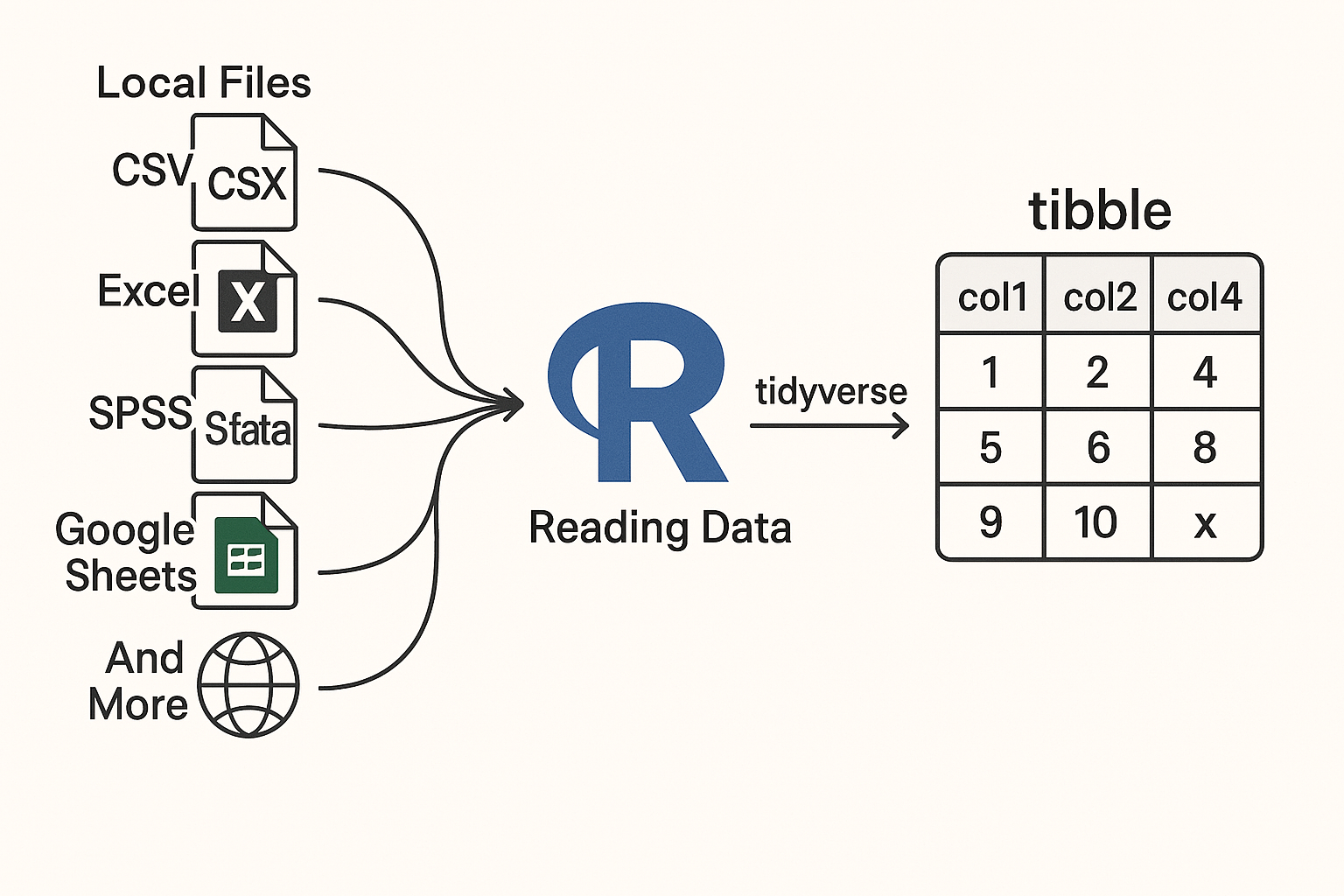
2. Introduction to Reading Data into R
Reading data into R is a foundational skill for any data analyst or scientist. R provides a rich ecosystem of packages to import data from a variety of sources and formats, making it easy to start your analysis.
Key Points
- R can read data from local files (CSV, Excel, SPSS, Stata, SAS, etc.), web APIs, Google Sheets, and more.
- The tidyverse ecosystem, especially packages like
readr,readxl,tibble, andhaven, streamlines data import and cleaning. - Specialized packages exist for cloud-based data (e.g.,
googlesheets4,googledrive), web scraping (rvest), and APIs (httr,jsonlite,xml2). - Tibbles (
tibblepackage) are modern data frames that improve usability and error handling.
2.1. Using tibble: Modern Data Frames
What is a tibble?
- A modern reimagining of the classic R
data.frame. - Does not change variable names or types automatically.
- Enhanced printing for large datasets.
- Forces you to handle problems early, leading to cleaner code.
Example: Creating a tibble
library(tibble)
data_tbl <- tibble(
  name = c("Alice", "Bob"),
  age = c(25, 30)
)
print(data_tbl)
Expected Output:
| name | age |
|---|---|
| Alice | 25 |
| Bob | 30 |
2.2. Reading CSV Files with readr
readrprovides fast and friendly functions for reading rectangular data (CSV, TSV, etc.).- Functions like
read_csv()andread_tsv()are commonly used.
Example: Reading a CSV file
library(readr)
data <- read_csv("data/sample.csv")
head(data)
Input (data/sample.csv):
name,age,city
Alice,25,Boston
Bob,30,Chicago
Expected Output:
| name | age | city |
|---|---|---|
| Alice | 25 | Boston |
| Bob | 30 | Chicago |
2.3. Reading Google Sheets with googlesheets4
- Access and manage Google Sheets directly from R.
- Useful for collaborative and cloud-based data.
Example: Reading a Google Sheet
library(googlesheets4)
sheet_url <- "https://docs.google.com/spreadsheets/d/your_sheet_id"
gs_data <- read_sheet(sheet_url)
head(gs_data)
Expected Output:
A tibble with the contents of the Google Sheet.
2.4. Reading Excel Files with readxl
- Read
.xlsand.xlsxfiles easily. - No external dependencies.
Example: Reading an Excel file
library(readxl)
excel_data <- read_excel("data/sample.xlsx")
head(excel_data)
Input (data/sample.xlsx):
| id | score |
|---|---|
| 1 | 88 |
| 2 | 92 |
Expected Output:
| id | score |
|---|---|
| 1 | 88 |
| 2 | 92 |
2.5. Accessing Google Drive Files with googledrive
- Manage and download files from Google Drive.
Example: Listing files in Google Drive
library(googledrive)
# Authenticate using a service account JSON file (replace with your file path)
drive_auth(path = "path/to/your-service-account.json")
drive_find(n_max = 5)
Expected Output:
A tibble listing up to 5 files from your Google Drive.
2.6. Importing Data from SPSS, Stata, SAS with haven
- Read data from statistical software formats.
Example: Reading a SAS file
library(haven)
sas_data <- read_sas("data/sample.sas7bdat")
head(sas_data)
Expected Output:
A tibble with the contents of the SAS file.
2.7. Reading JSON and XML Data
- Use
jsonlitefor JSON andxml2for XML data. - Common for web APIs and semi-structured data.
Example: Reading JSON
library(jsonlite)
json_data <- fromJSON('{"name": "Alice", "age": 25}')
print(json_data)
Expected Output:
| name | age |
|---|---|
| Alice | 25 |
Example: Reading XML
library(xml2)
xml <- read_xml("<person><name>Alice</name><age>25</age></person>")
xml_text(xml_find_first(xml, ".//name"))
Expected Output:
"Alice"
2.8. Web Scraping with rvest
- Extract data from web pages.
Example: Scraping a table from a webpage
library(rvest)
url <- "https://example.com/table"
page <- read_html(url)
table <- html_table(html_node(page, "table"))
head(table)
Expected Output:
A data frame with the table's contents.
2.9. Accessing APIs with httr
- Interact with web APIs to retrieve data.
Example: GET request to an API
library(httr)
response <- GET("https://api.example.com/data")
content <- content(response, "parsed")
print(content)
Expected Output:
A list or data frame with the API response data.
3. Introduction to Data Tidying Packages
- Data and information are stored in many formats on computers and the Internet.
- After importing data into R, the next step is to tidy or wrangle the data for analysis.
- Several R packages help convert untidy data into a flexible, usable tidy format.
**Key Packages for Data Tidying**
| Package | Main Purpose | Example Functions | Typical Use Case |
|---|---|---|---|
| dplyr | Data manipulation (filter, select, mutate, etc.) | mutate, select, filter, summarize, arrange |
Transforming and summarizing data |
| tidyr | Reshaping and tidying data | pivot_longer, pivot_wider, separate, unite |
Making data tidy (columns = variables, rows = obs) |
| janitor | Cleaning dirty data | clean_names, remove_empty, tabyl |
Cleaning column names, removing empty rows/cols |
| forcats | Handling categorical variables (factors) | fct_reorder, fct_lump, fct_recode |
Reordering, lumping, and recoding factor levels |
| stringr | String manipulation | str_detect, str_replace, str_split |
Cleaning and extracting text |
| lubridate | Dates and times | ymd, mdy, year, month, wday |
Parsing and manipulating date/time data |
| glue | String interpolation | glue |
Building dynamic strings |
| skimr | Data summarization | skim |
Quick, tidy summaries of data frames |
| tidytext | Text mining in tidy format | unnest_tokens, bind_tf_idf |
Analyzing and tidying text data |
| purrr | Functional programming and iteration | map, map_df, map_chr |
Applying functions to lists/vectors |
**Visual Workflow for Data Tidying Packages**
flowchart TD
    A[Import Data (readr, readxl, haven,
        googlesheets4, jsonlite)] --> B[Initial Cleaning janitor)]
    B --> C[Tidy Data Structure<br/>(tidyr)]
    C --> D[Data Manipulation<br/>(dplyr)]
    D --> E[Categorical Data<br/>(forcats)]
    D --> F[String Operations<br/>(stringr)]
    D --> G[Date/Time Handling<br/>(lubridate)]
    D --> H[Dynamic Strings<br/>(glue)]
    D --> I[Summarize Data<br/>(skimr)]
    D --> J[Text Analysis<br/>(tidytext)]
    D --> K[Functional Programming<br/>(purrr)]
**Step-by-Step Workflow**
Import Data
Use packages such asreadr,readxl,haven,googlesheets4,jsonlite.Initial Cleaning
Clean column names, remove empty rows/columns withjanitor.Tidy Data Structure
Reshape and organize data usingtidyr.Data Manipulation
Transform and summarize data withdplyr.Work with Categorical Data
Manage factors usingforcats.Work with Strings
Clean and manipulate text withstringr.Work with Dates and Times
Parse and handle date/time data withlubridate.Dynamic String Construction
Build dynamic strings usingglue.Summarize Data
Get quick summaries withskimr.Text Data Analysis
Analyze text data usingtidytext.Functional Programming and Iteration
Apply functions to lists/vectors withpurrr.
4. Data Visualization: An Introduction for Beginners
- Data visualization is a key part of any data science project.
- After tidying your data, you’ll want to explore it visually to better understand patterns, trends, and outliers.
- Creating basic plots helps you quickly get a sense of your dataset.
- Well-designed visualizations are essential for communicating your findings to others.
- R provides several powerful packages to help you create both simple and advanced visualizations.
Key Packages for Data Visualization
ggplot2
- The most important package for creating plots in R.
- Lets you build a wide variety of charts (scatterplots, bar charts, histograms, etc.) with a consistent and flexible syntax.
- Based on the "Grammar of Graphics"—you map your data to visual elements and ggplot2 handles the details.
- Highly customizable for publication-quality graphics.
- Essential for any data science or analytics work in R.
kableExtra
- While plots are important, tables are also a great way to present information.
- kableExtra builds on top of the knitr::kable() function to let you create beautiful, complex tables.
- Offers a ggplot2-inspired syntax for customizing tables, adding color, borders, footnotes, and more.
ggrepel
- An extension for ggplot2 that helps prevent text labels from overlapping in your plots.
- Makes your charts easier to read by automatically adjusting label positions.
cowplot
- Helps you polish and arrange your ggplot2 plots for publication.
- Provides themes, alignment tools, and functions to combine multiple plots or add annotations.
patchwork
- Another package for combining multiple ggplot2 plots into a single figure.
- Makes it easy to arrange plots side-by-side or in grids, perfect for comparisons.
gganimate
- Allows you to add animation to your ggplot2 plots.
- Useful for showing changes over time or creating engaging, dynamic visualizations.
- Extends the grammar of graphics to include animation, making it easy to animate transitions and data changes.
5. Data Modeling: An Introduction for Beginners
- After reading, tidying, and exploring your data, the next step is data modeling—using your data to answer questions or make predictions.
- Data modeling includes both predictive modeling (like machine learning) and inferential statistics (like hypothesis testing).
- R provides several tidy and user-friendly packages for modeling, making the process more consistent and approachable.
Key Packages and Ecosystems for Data Modeling
tidymodels ecosystem
- A collection of packages for building, evaluating, and tuning predictive models and machine learning workflows.
- Handles data splitting, preprocessing, model fitting, and performance assessment in a unified way.
- Lets you use a wide range of algorithms from different R packages with a consistent, tidy syntax.
broom
- Converts statistical model outputs (like those from
lm(),glm(), etc.) into tidy data frames. - Makes it easy to extract and work with model results for reporting and visualization.
- Converts statistical model outputs (like those from
infer
- Provides a tidy, consistent grammar for statistical inference (e.g., t-tests, permutation tests).
- Standardizes syntax for different statistical tests, making inferential analysis easier to learn and apply.
tidyverts (tsibble, feasts, fable)
- A suite of packages for tidy time series analysis and forecasting.
- tsibble: A time-series version of a tibble, designed for organizing and wrangling temporal data.
- feasts: Tools for analyzing and extracting features from time series data.
- fable: Provides a range of forecasting models and tools for evaluating and visualizing forecasts, all within a tidy workflow.
Workflow Flow:
- Prepare your data (tidy, clean, and explore).
- Choose the right modeling approach (predictive, inferential, or time series).
- Use tidymodels for machine learning and predictive modeling.
- Use broom and infer for tidy statistical inference and hypothesis testing.
- Use tidyverts packages for time series analysis and forecasting.
- Interpret and communicate your results using tidy outputs and visualizations.