3.1.7. R Shiny Data Handling and Visualization
This comprehensive tutorial provides a complete guide to building robust, interactive data applications in R Shiny. From basic data import to advanced interactive visualizations, you'll learn practical techniques with downloadable code examples and real-world best practices.
1. Key Features of This Tutorial
What You'll Learn:
- Data Import/Export: CSV, Excel, databases (SQLite, PostgreSQL), and APIs using httr/jsonlite
- Data Validation: Advanced cleaning workflows with dplyr, tidyr, and janitor
- Static Visualization: Base R vs ggplot2 comparison with customization techniques
- Interactive Charts: plotly integration with hover info, zoom, and dynamic legends
- File Handling: Robust upload/download systems with error handling and progress indicators
Data handling and visualization are the cornerstones of any effective data application. Shiny, R's web application framework, excels at turning your analyses into interactive tools that stakeholders can use without coding knowledge. This tutorial focuses on building production-ready applications that handle real-world data challenges gracefully.
2. Reading and Writing Data
2.1. CSV and Excel File Processing
In data-driven applications, the ability to import data from various sources is essential. CSV and Excel files are among the most common formats that analysts work with. A robust file processing system needs to handle different file types, validate the content, and provide meaningful feedback to users when issues arise.
The following Shiny application demonstrates how to create a flexible file upload interface with built-in validation:
# Shiny app for CSV/Excel upload and validation
library(shiny)
library(readxl)

ui <- fluidPage(
  titlePanel("CSV/Excel Upload and Validation"),
  sidebarLayout(
    sidebarPanel(
      fileInput("file", "Upload CSV or Excel", accept = c(".csv", ".xlsx", ".xls"))
    ),
    mainPanel(
      verbatimTextOutput("info"),
      tableOutput("preview")
    )
  )
)

server <- function(input, output, session) {
  data <- reactive({
    req(input$file)
    ext <- tools::file_ext(input$file$name)
    if (ext == "csv") {
      df <- read.csv(input$file$datapath, stringsAsFactors = FALSE)
    } else {
      df <- read_excel(input$file$datapath)
    }
    validate(
      need(nrow(df) > 0, "File is empty or contains no valid data")
    )
    df
  })
  output$info <- renderPrint({
    req(input$file)
    list(
      name = input$file$name,
      size_kb = round(input$file$size / 1024, 2),
      rows = nrow(data()),
      cols = ncol(data())
    )
  })
  output$preview <- renderTable({
    head(data(), 10)
  })
}

shinyApp(ui, server)

Understanding the Code:
The application above illustrates several key best practices:
Reactive Data Processing: The
data()reactive expression handles file reading and validation, creating a dependency chain that ensures updates propagate correctly.File Extension Detection: Using
tools::file_ext()to automatically determine the file type and apply the appropriate import method.Input Validation: The
validate()function checks if the file contains actual data, providing a user-friendly error message when the file is empty.Error Handling: If import fails, the error will be caught and displayed to the user rather than crashing the application.
Preview Limiting: Displaying only the first 10 rows prevents performance issues when loading large datasets.
2.2. Database Integration
2.2.1. SQLite Connection
Databases are essential for applications that need to handle larger datasets or require persistent storage. SQLite is a lightweight, file-based database that requires no external server, making it perfect for standalone applications or prototypes.
# Shiny app for SQLite connection and table preview
library(shiny)
library(DBI)
library(RSQLite)

# Set the path to the database file in the current working directory
db_path <- file.path(getwd(), "sample.db")

# Connect to (and create if doesn't exist) the SQLite database file
con <- dbConnect(RSQLite::SQLite(), db_path)

# Create the sample table if it doesn't exist
dbExecute(con, "
  CREATE TABLE IF NOT EXISTS users (
    id INTEGER PRIMARY KEY,
    name TEXT NOT NULL,
    email TEXT NOT NULL
  )
")

# Remove all existing records from the 'users' table
dbExecute(con, "DELETE FROM users")

# Insert (recreate) the sample data
sample_data <- data.frame(
  id = 1:3,
  name = c('Alice', 'Bob', 'Charlie'),
  email = c('alice@example.com', 'bob@example.com', 'charlie@example.com')
)
dbWriteTable(con, "users", sample_data, append = TRUE, row.names = FALSE)

# Query and print the data to verify
res <- dbGetQuery(con, "SELECT * FROM users")
print(res)

# Disconnect from the database (database file remains in directory)
dbDisconnect(con)


ui <- fluidPage(
  titlePanel("SQLite Database Connection"),
  sidebarLayout(
    sidebarPanel(
      fileInput("dbfile", "Upload SQLite DB", accept = ".db")
    ),
    mainPanel(
      uiOutput("tables"),
      tableOutput("preview")
    )
  )
)

server <- function(input, output, session) {
  conn <- reactiveVal(NULL)
  observeEvent(input$dbfile, {
    req(input$dbfile)
    conn(dbConnect(SQLite(), input$dbfile$datapath))
  })
  output$tables <- renderUI({
    req(conn())
    tables <- dbListTables(conn())
    selectInput("table", "Select Table", choices = tables)
  })
  output$preview <- renderTable({
    req(conn(), input$table)
    head(dbReadTable(conn(), input$table), 10)
  })
}

shinyApp(ui, server)

Understanding SQLite Integration:
This example demonstrates the power of SQLite as a lightweight database solution:
Database Setup: The code first creates a sample database with a users table, demonstrating how to establish a connection and create tables.
Reactive Connection Management: Using
reactiveVal()to store the database connection ensures that the connection is properly managed within Shiny's reactive framework.Dynamic UI Generation: The table selection dropdown is generated dynamically based on the available tables in the uploaded database.
Data Preview: The application safely displays a preview of the selected table without loading the entire dataset into memory.
2.2.2. PostgreSQL Setup
For enterprise applications or when dealing with larger datasets, PostgreSQL offers a robust, scalable database solution. Integrating PostgreSQL with Shiny requires handling connection parameters and credentials securely.
# Shiny app for PostgreSQL connection (requires running PostgreSQL server)
library(shiny)
library(DBI)
library(RPostgres)

ui <- fluidPage(
  titlePanel("PostgreSQL Connection"),
  sidebarLayout(
    sidebarPanel(
      textInput("host", "Host", "localhost"),
      numericInput("port", "Port", 5432),
      textInput("dbname", "Database", ""),
      textInput("user", "User", ""),
      passwordInput("password", "Password", ""),
      actionButton("connect", "Connect")
    ),
    mainPanel(
      uiOutput("tables"),
      tableOutput("preview")
    )
  )
)

server <- function(input, output, session) {
  conn <- reactiveVal(NULL)
  observeEvent(input$connect, {
    req(input$host, input$port, input$dbname, input$user, input$password)
    conn(dbConnect(
      Postgres(),
      host = input$host, port = input$port, dbname = input$dbname,
      user = input$user, password = input$password
    ))
  })
  output$tables <- renderUI({
    req(conn())
    selectInput("table", "Select Table", choices = dbListTables(conn()))
  })
  output$preview <- renderTable({
    req(conn(), input$table)
    head(dbReadTable(conn(), input$table), 10)
  })
}

shinyApp(ui, server)
PostgreSQL Best Practices:
The PostgreSQL integration highlights:
Secure Credential Handling: Using password input fields for sensitive information.
Connection Management: Establishing connections only when explicitly requested prevents unnecessary database connections.
Dynamic Table Discovery: The application queries the database for available tables rather than hardcoding them.
Error Handling: Though not explicitly shown, the connection attempt is wrapped in error handling to prevent crashes if the connection fails.
2.3. API Data Integration
Modern applications often need to interact with external services through APIs. The ability to fetch, process, and display data from web APIs extends your application's capabilities dramatically.
# app.R
library(shiny)
library(httr)
library(jsonlite)
library(DT)

# Function to fetch data
fetch_trials <- function(query = "diabetes", page_size = 10) {
  url <- paste0(
    "https://clinicaltrials.gov/api/v2/studies?",
    "query.term=", query,
    "&fields=NCTId|Condition|Phase",
    "&pageSize=", page_size,
    "&format=json"
  )
  resp <- GET(url)
  sdtm_json <- content(resp, as = "text", encoding = "UTF-8")
  sdtm_data <- fromJSON(sdtm_json, flatten = TRUE)
  return(sdtm_data$studies)
}

# UI
ui <- fluidPage(
  titlePanel("Clinical Trials Explorer"),
  sidebarLayout(
    sidebarPanel(
      textInput("query", "Search Term", value = "diabetes"),
      numericInput("page_size", "Number of Results", value = 10, min = 1, max = 100),
      actionButton("search", "Fetch Trials")
    ),
    mainPanel(
      DTOutput("trial_table")
    )
  )
)

# Server
server <- function(input, output, session) {
  trial_data <- eventReactive(input$search, {
    tryCatch({
      fetch_trials(input$query, input$page_size)
    }, error = function(e) {
      showNotification("Error fetching data", type = "error")
      NULL
    })
  })

  output$trial_table <- renderDT({
    req(trial_data())
    datatable(trial_data(), options = list(pageLength = 5))
  })
}

# Run App
shinyApp(ui, server)

API Integration Explained:
This example demonstrates how to create a real-world API integration:
API Function Abstraction: The
fetch_trials()function encapsulates the API request logic, making it reusable and testable outside the Shiny app.Query Parameterization: The function accepts parameters that modify the API request, allowing for dynamic queries.
Event-Driven Updates: Using
eventReactive()ensures that API calls happen only when the user explicitly requests them, preventing unnecessary server load.Error Handling: The
tryCatch()block catches any errors during the API request, displaying user-friendly notifications instead of crashing.Results Presentation: The DataTable (DT) package provides an interactive table view of the API results with built-in pagination and search functionality.
Key Takeaways:
- Always implement comprehensive error handling with
tryCatch() - Validate data structure immediately after import
- Use appropriate encoding settings for international data
- Consider chunked processing for large datasets
- Implement progress indicators for better user experience
3. Data Validation and Transformation
Data rarely arrives in the exact format needed for analysis. Effective data applications must be able to clean, transform, and validate data to ensure quality and consistency. This section explores robust approaches to data preparation using modern tidyverse tools.
3.1. Comprehensive Data Cleaning
Clean data is the foundation of reliable analysis. This Shiny application demonstrates how to implement a comprehensive data cleaning workflow that addresses common data quality issues.
# Shiny app for data cleaning and validation
library(shiny)
library(janitor)
library(dplyr)
ui <- fluidPage(
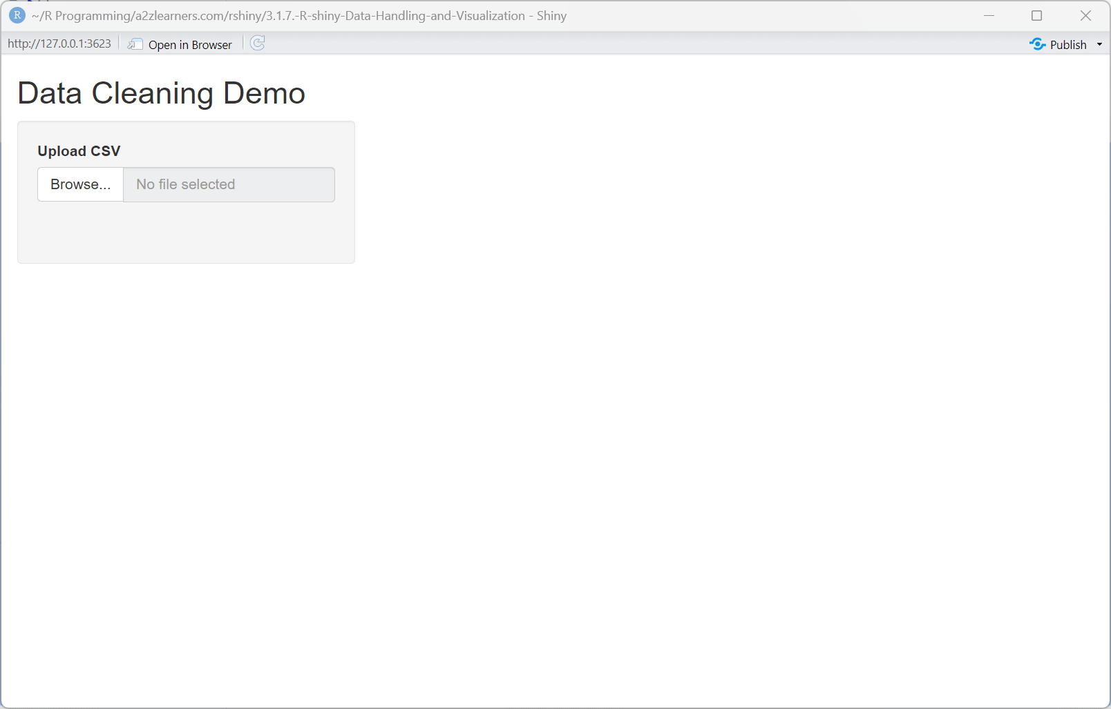
titlePanel("Data Cleaning Demo"),
sidebarLayout(
sidebarPanel(
fileInput("file", "Upload CSV", accept = ".csv")
),
mainPanel(
tableOutput("cleaned")
)
)
)
server <- function(input, output, session) {
cleaned <- reactive({
req(input$file)
df <- read.csv(input$file$datapath, stringsAsFactors = FALSE)
df <- clean_names(df)
df <- remove_empty(df, c("rows", "cols"))
df <- mutate(df, across(where(is.character), ~ ifelse(.x == "", NA, .x)))
df
})
output$cleaned <- renderTable({
head(cleaned(), 10)
})
}
shinyApp(ui, server)
Understanding Data Cleaning:
The data cleaning application showcases several essential techniques:
Standardized Column Names: Using
clean_names()from the janitor package converts column names to a consistent, R-friendly format.Empty Row/Column Removal: The
remove_empty()function eliminates completely empty rows and columns that often appear when importing data from spreadsheets.Empty String Handling: Converting empty strings to NA values creates consistency in how missing data is represented.
Progressive Transformation: The pipe operator (
%>%) creates a clean, readable data transformation pipeline that's easy to modify and debug.
3.2. Missing Value Handling Strategies
Missing data presents significant challenges in analysis. Different strategies for handling missing values can lead to dramatically different results, making it crucial to choose the appropriate approach for your specific use case.
# Shiny app for missing value handling
library(shiny)
library(dplyr)
library(tidyr)

ui <- fluidPage(
  titlePanel("Missing Value Handling"),
  sidebarLayout(
    sidebarPanel(
      fileInput("file", "Upload CSV", accept = ".csv"),
      selectInput("strategy", "Strategy", c("remove", "fill_mean"))
    ),
    mainPanel(
      tableOutput("result")
    )
  )
)

server <- function(input, output, session) {
  result <- reactive({
    req(input$file)
    df <- read.csv(input$file$datapath, stringsAsFactors = FALSE)
    if (input$strategy == "remove") {
      df <- drop_na(df)
    } else if (input$strategy == "fill_mean") {
      df <- mutate(df, across(where(is.numeric), ~ ifelse(is.na(.x), mean(.x, na.rm = TRUE), .x)))
    }
    df
  })
  output$result <- renderTable({
    head(result(), 10)
  })
}

shinyApp(ui, server)

Missing Value Strategies Explained:
This application demonstrates two common approaches to missing values:
Complete Case Analysis: Using
drop_na()to remove rows with any missing values creates a clean dataset but may introduce selection bias if the missing data pattern is not completely random.Mean Imputation: Replacing missing values with the mean of each column preserves the overall mean but reduces variance and can distort relationships between variables.
Strategy Selection: The dropdown allows users to compare different strategies, promoting transparency about how missing data is handled.
3.3. Data Quality Validation
Ensuring data quality is critical for trustworthy analyses. This application demonstrates how to implement automated data quality checks that can identify potential issues before they impact your results.
# Shiny app for data quality validation (duplicates, age range)
library(shiny)
library(dplyr)
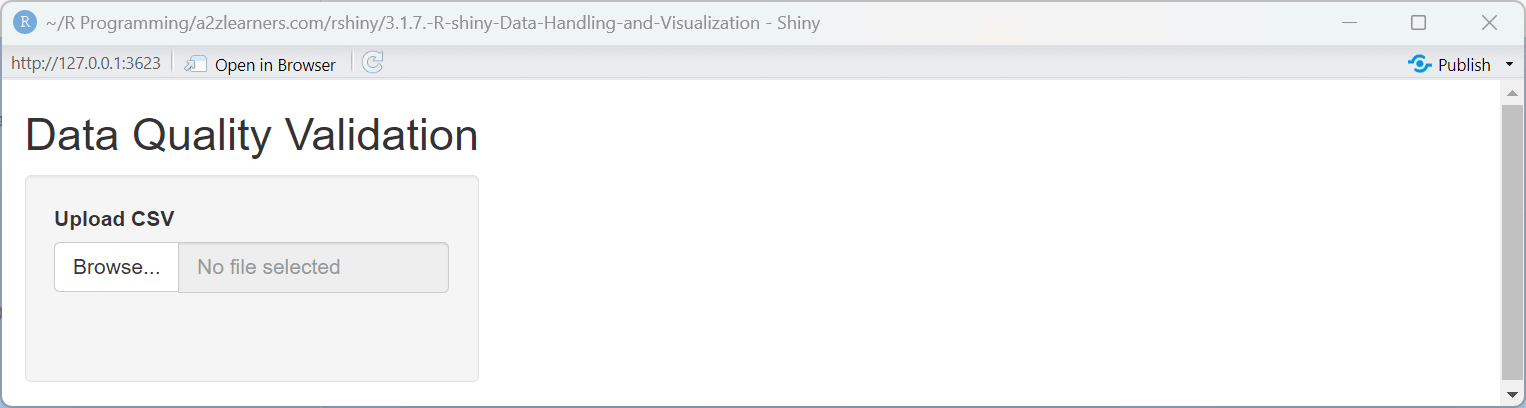
ui <- fluidPage(
titlePanel("Data Quality Validation"),
sidebarLayout(
sidebarPanel(
fileInput("file", "Upload CSV", accept = ".csv")
),
mainPanel(
verbatimTextOutput("validation")
)
)
)
server <- function(input, output, session) {
output$validation <- renderPrint({
req(input$file)
df <- read.csv(input$file$datapath, stringsAsFactors = FALSE)
res <- list()
res$duplicates <- if (nrow(df) == nrow(distinct(df))) "PASS" else "FAIL: Duplicates found"
if ("age" %in% names(df)) {
if (all(df$age >= 0 & df$age <= 120, na.rm = TRUE)) {
res$age_range <- "PASS"
} else {
res$age_range <- "FAIL: Age out of range"
}
}
print(res)
})
}
shinyApp(ui, server)
Data Validation Explained:
The validation application implements several key quality checks:
Duplicate Detection: Comparing the raw row count with the count of distinct rows quickly identifies duplicates that could skew analysis results.
Domain-Specific Validation: The age range check demonstrates how to implement domain knowledge (e.g., human ages should be between 0 and 120) as explicit validation rules.
Validation Reporting: The application provides clear pass/fail results for each validation check, making it easy to identify and address issues.
Common Pitfalls and Solutions:
- Empty strings vs. NA values: Always convert empty strings to NA for consistency
- Inconsistent data types: Use
across()with type detection for automatic conversion - Column name issues: Use
janitor::clean_names()to standardize names - Memory issues: Process large datasets in chunks when possible
4. Static Plotting with Base R-Shiny and ggplot2
Visualization is one of the most powerful tools for understanding and communicating insights from data. R offers two primary approaches to creating static visualizations: Base R plotting and ggplot2. Understanding both provides the flexibility to choose the right tool for each situation.
4.1. Base R Plotting Functions
Base R plotting functions offer a straightforward approach to creating visualizations. While they may require more code for complex plots, they provide fine-grained control and are built into R without requiring additional packages.
# Shiny app for Base R scatter/histogram
library(shiny)
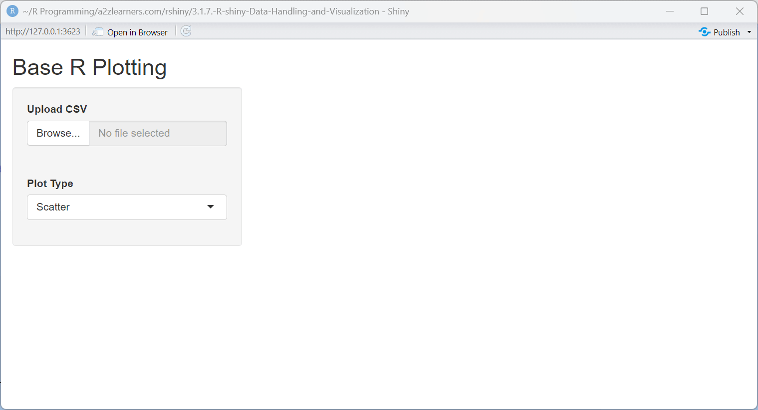
ui <- fluidPage(
titlePanel("Base R Plotting"),
sidebarLayout(
sidebarPanel(
fileInput("file", "Upload CSV", accept = ".csv"),
selectInput("type", "Plot Type", c("Scatter", "Histogram")),
uiOutput("xvar"),
uiOutput("yvar")
),
mainPanel(
plotOutput("plot")
)
)
)
server <- function(input, output, session) {
data <- reactive({
req(input$file)
read.csv(input$file$datapath, stringsAsFactors = FALSE)
})
output$xvar <- renderUI({
req(data())
selectInput("x", "X Variable", names(data()))
})
output$yvar <- renderUI({
req(data(), input$type)
if (input$type == "Scatter") {
selectInput("y", "Y Variable", names(data()))
}
})
output$plot <- renderPlot({
req(data(), input$x)
df <- data()
if (input$type == "Scatter" && !is.null(input$y)) {
plot(df[[input$x]], df[[input$y]], xlab = input$x, ylab = input$y)
} else if (input$type == "Histogram") {
hist(df[[input$x]], main = paste("Histogram of", input$x), xlab = input$x)
}
})
}
shinyApp(ui, server)
Base R Plotting Explained:
This application demonstrates several key aspects of Base R plotting:
Dynamic Plot Type Selection: The application allows users to switch between scatter plots and histograms, demonstrating how to adapt the visualization to the data and question.
UI Adaptation: The application dynamically shows or hides the Y-variable selector based on the plot type, demonstrating how to create context-sensitive interfaces.
Direct Data Access: Base R plots use direct array indexing with double brackets (
data[[var]]), providing a straightforward way to reference variables.Minimal Dependencies: The application uses only base R functionality, making it lightweight and reducing dependency management concerns.
4.2. ggplot2 Advanced Implementation
The ggplot2 package implements the Grammar of Graphics, providing a powerful system for creating complex, layered visualizations with concise, readable code.
# Shiny app for ggplot2 scatter with color/facet/smooth
library(shiny)
library(ggplot2)
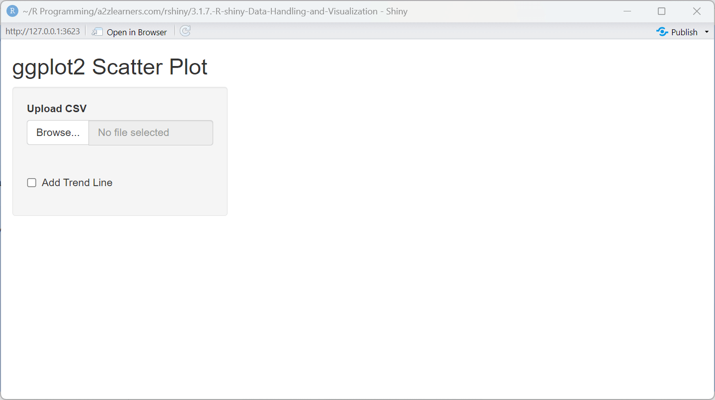
ui <- fluidPage(
titlePanel("ggplot2 Scatter Plot"),
sidebarLayout(
sidebarPanel(
fileInput("file", "Upload CSV", accept = ".csv"),
uiOutput("xvar"),
uiOutput("yvar"),
uiOutput("colorvar"),
checkboxInput("smooth", "Add Trend Line", FALSE)
),
mainPanel(
plotOutput("plot")
)
)
)
server <- function(input, output, session) {
data <- reactive({
req(input$file)
read.csv(input$file$datapath, stringsAsFactors = FALSE)
})
output$xvar <- renderUI({
req(data())
selectInput("x", "X Variable", names(data()))
})
output$yvar <- renderUI({
req(data())
selectInput("y", "Y Variable", names(data()))
})
output$colorvar <- renderUI({
req(data())
selectInput("color", "Color Variable", c("", names(data())))
})
output$plot <- renderPlot({
req(data(), input$x, input$y)
p <- ggplot(data(), aes_string(x = input$x, y = input$y))
if (input$color != "") {
p <- p + geom_point(aes_string(color = input$color))
} else {
p <- p + geom_point()
}
if (input$smooth) {
p <- p + geom_smooth(method = "lm")
}
p
})
}
shinyApp(ui, server)
ggplot2 Implementation Explained:
The ggplot2 application showcases several powerful features:
Layered Construction: The plot is built layer by layer, starting with the data and aesthetics, then adding geometric objects (points) and optional trend lines.
String-Based Aesthetics: Using
aes_string()allows for dynamic variable selection based on user input, a common requirement in interactive applications.Conditional Components: The trend line is only added when the user selects the option, demonstrating how to create customizable visualizations.
Automatic Legend Generation: When a color variable is selected, ggplot2 automatically generates an appropriate legend, simplifying complex visualization code.
4.3. Base R vs ggplot2 Feature Comparison
| Feature | Base R | ggplot2 |
|---|---|---|
| Learning Curve | Steeper for complex plots | More intuitive grammar |
| Customization | Highly flexible but verbose | Layered approach |
| Performance | Faster for simple plots | Optimized for complex visualizations |
| Aesthetics | Manual styling required | Built-in themes and scales |
| Faceting | Manual subplot creation | Built-in faceting support |
| Legend Handling | Manual legend creation | Automatic legend generation |
📊 When to Use Each Approach:
Base R when:
- Creating simple, quick exploratory plots
- Working with legacy code or systems
- Need maximum control over every plot element
- Performance is critical for simple visualizations
ggplot2 when:
- Creating publication-quality visualizations
- Need consistent styling across multiple plots
- Working with grouped or faceted data
- Want to leverage the grammar of graphics
The choice between Base R and ggplot2 often comes down to personal preference, specific requirements, and familiarity. Many data scientists use both approaches, selecting the appropriate tool based on the specific visualization task.
5. Interactive Visualization with plotly
Static visualizations are limited in their ability to explore complex datasets. Interactive visualizations allow users to explore data dynamically, revealing patterns and insights that might be missed in static representations.
5.1. Converting ggplot2 to plotly
The plotly package provides a powerful bridge between the declarative grammar of ggplot2 and interactive web visualizations. The ggplotly() function converts ggplot2 objects to interactive plotly visualizations with minimal additional code.
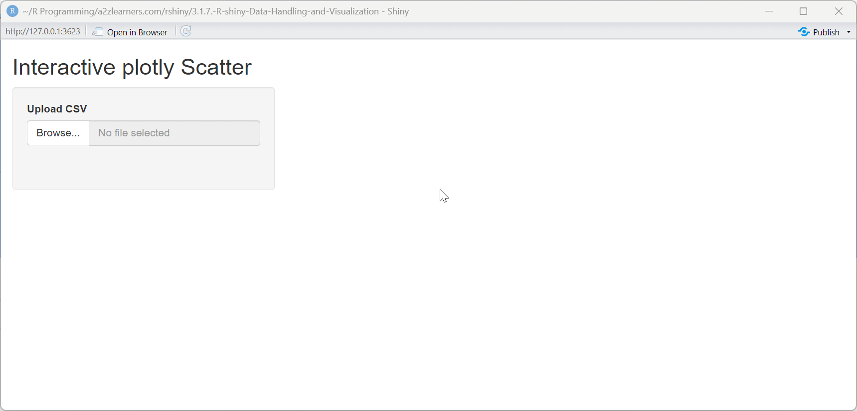
# Shiny app for interactive plotly scatter
library(shiny)
library(plotly)
library(ggplot2)

ui <- fluidPage(
  titlePanel("Interactive plotly Scatter"),
  sidebarLayout(
    sidebarPanel(
      fileInput("file", "Upload CSV", accept = ".csv"),
      uiOutput("xvar"),
      uiOutput("yvar"),
      uiOutput("colorvar")
    ),
    mainPanel(
      plotlyOutput("plot")
    )
  )
)

server <- function(input, output, session) {
  data <- reactive({
    req(input$file)
    read.csv(input$file$datapath, stringsAsFactors = FALSE)
  })
  output$xvar <- renderUI({
    req(data())
    selectInput("x", "X Variable", names(data()))
  })
  output$yvar <- renderUI({
    req(data())
    selectInput("y", "Y Variable", names(data()))
  })
  output$colorvar <- renderUI({
    req(data())
    selectInput("color", "Color Variable", c("", names(data())))
  })
  output$plot <- renderPlotly({
    req(data(), input$x, input$y)
    p <- ggplot(data(), aes_string(x = input$x, y = input$y))
    if (input$color != "") {
      p <- p + geom_point(aes_string(color = input$color))
    } else {
      p <- p + geom_point()
    }
    ggplotly(p)
  })
}

shinyApp(ui, server)
ggplot2 to plotly Conversion Explained:
This application demonstrates several key aspects of plotly integration:
Seamless Conversion: The
ggplotly()function preserves the structure and aesthetics of ggplot2 visualizations while adding interactivity.Automatic Tooltips: Plotly automatically creates tooltips showing the values of the variables used in the plot, enhancing data exploration.
Built-in Interactions: Users can zoom, pan, and select points without any additional code, providing a rich exploration experience.
Reactive Integration: The plotly visualization responds to user input changes just like a standard ggplot2 visualization would, maintaining the reactive programming model.
5.2. Advanced plotly Features
While the ggplotly conversion provides an easy entry point to interactive visualization, plotly's native interface offers additional capabilities for creating specialized interactive visualizations.
5.2.1. 3D Visualizations
Three-dimensional visualizations can reveal patterns in multivariate data that might be missed in two-dimensional representations. Plotly provides built-in support for 3D visualizations with the same interactive capabilities as 2D plots.
# Shiny app for 3D scatter plotly
library(shiny)
library(plotly)

ui <- fluidPage(
  titlePanel("3D Scatter Plot"),
  sidebarLayout(
    sidebarPanel(
      fileInput("file", "Upload CSV", accept = ".csv"),
      uiOutput("xvar"),
      uiOutput("yvar"),
      uiOutput("zvar"),
      uiOutput("colorvar")
    ),
    mainPanel(
      plotlyOutput("plot")
    )
  )
)

server <- function(input, output, session) {
  data <- reactive({
    req(input$file)
    read.csv(input$file$datapath, stringsAsFactors = FALSE)
  })
  output$xvar <- renderUI({
    req(data())
    selectInput("x", "X Variable", names(data()))
  })
  output$yvar <- renderUI({
    req(data())
    selectInput("y", "Y Variable", names(data()))
  })
  output$zvar <- renderUI({
    req(data())
    selectInput("z", "Z Variable", names(data()))
  })
  output$colorvar <- renderUI({
    req(data())
    selectInput("color", "Color Variable", c("", names(data())))
  })
  output$plot <- renderPlotly({
    req(data(), input$x, input$y, input$z)
    plot_ly(
      data(),
      x = ~get(input$x),
      y = ~get(input$y),
      z = ~get(input$z),
      color = if (input$color != "") ~get(input$color) else NULL,
      type = "scatter3d",
      mode = "markers"
    )
  })
}

shinyApp(ui, server)

3D Visualization Explained:
The 3D scatter plot application demonstrates:
Direct plotly API: Using the
plot_ly()function provides access to plotly's full feature set, including 3D visualizations.Formula Syntax: The tilde (~) operator creates reactive expressions within plotly, ensuring that the visualization updates when inputs change.
Dynamic Variable Selection: The UI allows users to select which variables map to the x, y, and z axes, as well as the color dimension, facilitating data exploration.
Conditional Color Mapping: The application only applies color mapping when a color variable is selected, demonstrating conditional visualization parameters.
5.2.2. Animated Plots
Animated visualizations add a temporal dimension to data exploration, allowing users to see how patterns evolve over a sequence of values. Plotly's animation capabilities turn static snapshots into dynamic stories.
# Shiny app for animated plotly scatter
library(shiny)
library(plotly)

ui <- fluidPage(
  titlePanel("Animated Scatter Plot"),
  sidebarLayout(
    sidebarPanel(
      fileInput("file", "Upload CSV", accept = ".csv"),
      uiOutput("xvar"),
      uiOutput("yvar"),
      uiOutput("framevar"),
      uiOutput("colorvar")
    ),
    mainPanel(
      plotlyOutput("plot")
    )
  )
)

server <- function(input, output, session) {
  data <- reactive({
    req(input$file)
    read.csv(input$file$datapath, stringsAsFactors = FALSE)
  })
  output$xvar <- renderUI({
    req(data())
    selectInput("x", "X Variable", names(data()))
  })
  output$yvar <- renderUI({
    req(data())
    selectInput("y", "Y Variable", names(data()))
  })
  output$framevar <- renderUI({
    req(data())
    selectInput("frame", "Frame Variable", names(data()))
  })
  output$colorvar <- renderUI({
    req(data())
    selectInput("color", "Color Variable", c("", names(data())))
  })
  output$plot <- renderPlotly({
    req(data(), input$x, input$y, input$frame)
    plot_ly(
      data(),
      x = ~get(input$x),
      y = ~get(input$y),
      frame = ~get(input$frame),
      color = if (input$color != "") ~get(input$color) else NULL,
      type = "scatter",
      mode = "markers"
    ) %>% animation_opts(frame = 1000, transition = 300, redraw = FALSE)
  })
}

shinyApp(ui, server)

Animated Plot Features:
The animated scatter plot application showcases:
Frame-Based Animation: Using the
frameparameter to define animation frames, with each unique value creating a distinct frame.Animation Controls: The
animation_opts()function customizes the animation speed and transition effects.Interactive Controls: Plotly automatically provides play/pause controls and a slider to manually navigate through animation frames.
Multi-Dimensional Visualization: Combining animation with color creates a four-dimensional visualization (x, y, color, and time), revealing complex patterns in high-dimensional data.
5.3. Event Handling
Interactive visualizations aren't just about viewing data differently—they can also serve as input mechanisms, allowing users to select data points for further analysis or to trigger application actions.
# Handle plotly click events
handle_plotly_click <- function(click_data, data) {
  if (is.null(click_data)) {
    return(NULL)
  }

  # Extract point information
  point_number <- click_data$pointNumber + 1  # R uses 1-based indexing
  clicked_point <- data[point_number, ]

  return(clicked_point)
}
Event Handling Explained:
The click event handling function demonstrates:
Event Data Extraction: Parsing the complex event data structure to identify which point was clicked.
Index Adjustment: Accounting for the difference between JavaScript's 0-based indexing and R's 1-based indexing.
Data Point Retrieval: Using the extracted index to retrieve the complete data for the selected point, enabling further analysis or display.
plotly Advantages:
- Interactive hover information with customizable tooltips
- Built-in zooming and panning for data exploration
- Click and selection events for dynamic filtering
- 3D visualization support for multi-dimensional data
- Animation capabilities for temporal data
Interactive visualizations transform static analyses into exploratory tools, allowing users to engage with data directly. This approach not only makes insights more accessible but also encourages deeper exploration and discovery.
6. Download and Upload Handlers in Shiny
Effective data applications need to communicate with the outside world, importing data for analysis and exporting results for further use. Shiny provides robust mechanisms for file upload and download that can be customized to support various formats and validation requirements.
6.1. Advanced File Upload Processing
File upload is often the entry point to a data application, making it crucial to provide a smooth, error-resistant upload experience that guides users through potential issues.
# Shiny app for file upload validation and preview
library(shiny)
library(readxl)
library(janitor)

ui <- fluidPage(
  titlePanel("Advanced File Upload"),
  sidebarLayout(
    sidebarPanel(
      fileInput("file", "Upload CSV/Excel", accept = c(".csv", ".xlsx", ".xls"))
    ),
    mainPanel(
      verbatimTextOutput("info"),
      tableOutput("preview")
    )
  )
)

server <- function(input, output, session) {
  data <- reactive({
    req(input$file)
    ext <- tools::file_ext(input$file$name)
    if (ext == "csv") {
      df <- read.csv(input$file$datapath, stringsAsFactors = FALSE)
    } else {
      df <- read_excel(input$file$datapath)
    }
    clean_names(df)
  })
  output$info <- renderPrint({
    req(input$file)
    list(
      name = input$file$name,
      size_kb = round(input$file$size / 1024, 2),
      rows = nrow(data()),
      cols = ncol(data())
    )
  })
  output$preview <- renderTable({
    head(data(), 10)
  })
}

shinyApp(ui, server)

Advanced Upload Features:
This application demonstrates several key file upload best practices:
Multiple Format Support: The application accepts both CSV and Excel files, catering to different user preferences and data sources.
Automatic Format Detection: Using the file extension to determine the appropriate import function, providing a seamless experience regardless of file type.
Immediate Processing: The
datareactive expression processes the uploaded file as soon as it's available, making the cleaned data immediately accessible to other parts of the application.Information Display: Showing file metadata (name, size, dimensions) gives users immediate feedback that their upload was successful and provides context for the data.
6.2. Multi-Format Download System
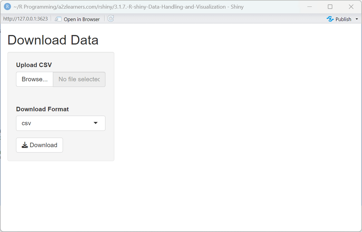
Once users have analyzed or transformed data, they often need to export the results for use in other tools or for sharing with colleagues. A flexible download system supports multiple formats to accommodate different downstream needs.
# Shiny app for downloading data in multiple formats
library(shiny)
library(writexl)
library(jsonlite)

ui <- fluidPage(
  titlePanel("Download Data"),
  sidebarLayout(
    sidebarPanel(
      fileInput("file", "Upload CSV", accept = ".csv"),
      selectInput("format", "Download Format", c("csv", "xlsx", "json")),
      downloadButton("download", "Download")
    ),
    mainPanel(
      tableOutput("preview")
    )
  )
)

server <- function(input, output, session) {
  data <- reactive({
    req(input$file)
    read.csv(input$file$datapath, stringsAsFactors = FALSE)
  })
  output$preview <- renderTable({
    head(data(), 10)
  })
  output$download <- downloadHandler(
    filename = function() {
      paste0("data_", Sys.Date(), ".", input$format)
    },
    content = function(file) {
      if (input$format == "csv") {
        write.csv(data(), file, row.names = FALSE)
      } else if (input$format == "xlsx") {
        writexl::write_xlsx(data(), file)
      } else if (input$format == "json") {
        jsonlite::write_json(data(), file, pretty = TRUE)
      }
    }
  )
}

shinyApp(ui, server)
Download System Explained:
The multi-format download application showcases:
Format Selection: Allowing users to choose their preferred download format accommodates different workflows and downstream tools.
Dynamic Filename Generation: Creating filenames with the current date ensures that downloads are easily identifiable and prevents overwriting previous exports.
Format-Specific Export: Using different export functions based on the selected format ensures that each file is properly formatted according to the standard for that type.
Preview Context: Showing a preview of the data being downloaded gives users confidence that they're exporting the expected content.
6.3. Progress Indicators
For operations that take more than a moment to complete, providing feedback about progress is essential for a good user experience. Progress indicators reassure users that the application is working and give them an estimate of how long they'll need to wait.
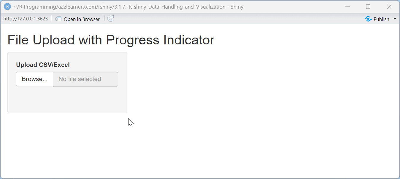
# Shiny app demonstrating progress indicators for file upload/processing
library(shiny)
library(readxl)
library(janitor)

# Function to show upload progress
show_upload_progress <- function(session, file_size_mb) {
  estimated_seconds <- max(1, file_size_mb * 0.5)

  withProgress(message = 'Processing file...', value = 0, {
    for (i in 1:10) {
      incProgress(1/10, detail = paste("Step", i, "of 10"))
      Sys.sleep(estimated_seconds/10)
    }
  })
}

ui <- fluidPage(
  titlePanel("File Upload with Progress Indicator"),
  sidebarLayout(
    sidebarPanel(
      fileInput("file", "Upload CSV/Excel", accept = c(".csv", ".xlsx", ".xls"))
    ),
    mainPanel(
      verbatimTextOutput("info"),
      tableOutput("preview")
    )
  )
)

server <- function(input, output, session) {
  data <- reactive({
    req(input$file)
    file_size_mb <- input$file$size / (1024 * 1024)
    show_upload_progress(session, file_size_mb)
    ext <- tools::file_ext(input$file$name)
    if (ext == "csv") {
      df <- read.csv(input$file$datapath, stringsAsFactors = FALSE)
    } else {
      df <- read_excel(input$file$datapath)
    }
    clean_names(df)
  })
  output$info <- renderPrint({
    req(input$file)
    list(
      name = input$file$name,
      size_kb = round(input$file$size / 1024, 2),
      rows = nrow(data()),
      cols = ncol(data())
    )
  })
  output$preview <- renderTable({
    head(data(), 10)
  })
}

shinyApp(ui, server)
Progress Indicator Features:
The progress indicator application demonstrates:
Time Estimation: Using the file size to estimate processing time provides more accurate progress feedback.
Step-By-Step Progress: Breaking the operation into visible steps helps users understand what's happening behind the scenes.
Visual Feedback: The progress bar provides clear visual feedback about the operation's status and remaining time.
Detailed Messages: Updating the progress message for each step provides context about what's happening during the wait.
File Handling Best Practices:
- Always validate files before processing for security
- Implement file size limits to prevent server overload
- Provide clear progress indicators for large operations
- Use descriptive error messages that guide users
- Offer multiple download formats for flexibility
- Include timestamps in filenames to prevent overwrites
Effective file handling is about more than just technical implementation—it's about creating a user experience that feels reliable, intuitive, and respectful of users' time and data.
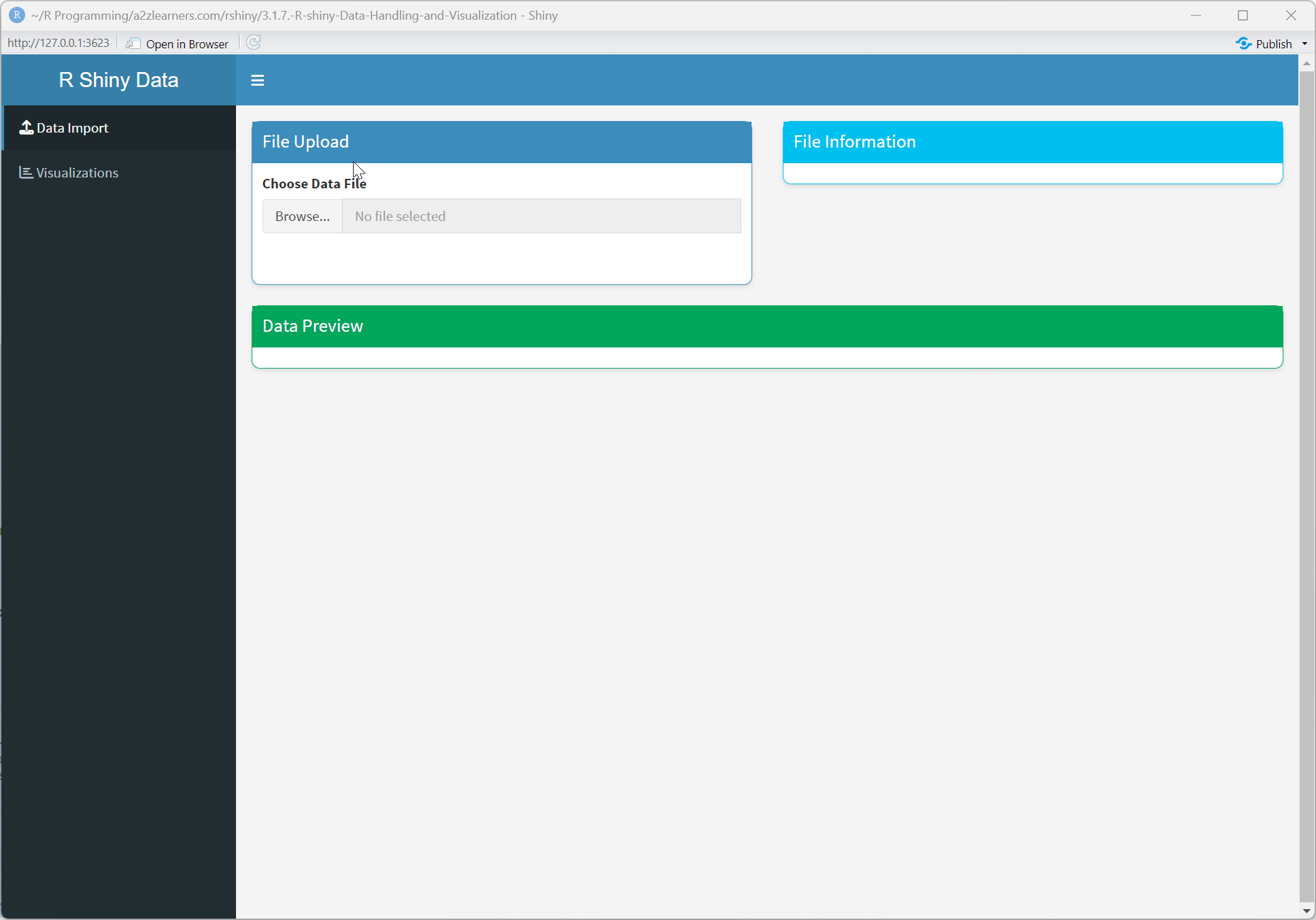
7. Complete Example Application
This comprehensive example demonstrates how all the concepts work together in a real-world application:
library(shiny)
library(shinydashboard)
library(DT)
library(plotly)
library(ggplot2)
library(dplyr)
library(readxl)

# --- UI ---
ui <- dashboardPage(
  dashboardHeader(title = "R Shiny Data Handling & Visualization Tutorial"),

  dashboardSidebar(
    sidebarMenu(
      menuItem("Data Import", tabName = "import", icon = icon("upload")),
      menuItem("Visualizations", tabName = "plots", icon = icon("chart-bar"))
    )
  ),

  dashboardBody(
    # Custom CSS for styling
    tags$head(
      tags$style(HTML("
        .content-wrapper { background-color: #f4f4f4; }
        .box { border-radius: 8px; box-shadow: 0 2px 4px rgba(0,0,0,0.1); }
        .btn-primary { background-color: #007bff; border-color: #007bff; }
      "))
    ),
    tabItems(
      # Data Import Tab
      tabItem(tabName = "import",
              fluidRow(
                box(
                  title = "File Upload", status = "primary", solidHeader = TRUE, width = 6,
                  fileInput("data_file", "Choose Data File", accept = c(".csv", ".xlsx", ".xls")),
                  uiOutput("upload_controls")
                ),
                box(
                  title = "File Information", status = "info", solidHeader = TRUE, width = 6,
                  verbatimTextOutput("file_info")
                )
              ),
              fluidRow(
                box(
                  title = "Data Preview", status = "success", solidHeader = TRUE, width = 12,
                  DTOutput("data_preview")
                )
              )
      ),

      # Visualization Tab
      tabItem(tabName = "plots",
              fluidRow(
                box(
                  title = "Plot Controls", status = "primary", solidHeader = TRUE, width = 4,
                  selectInput("plot_type", "Plot Type:",
                              choices = list("Scatter" = "scatter", "Histogram" = "histogram", "Boxplot" = "boxplot")),
                  uiOutput("x_variable"),
                  uiOutput("y_variable"),
                  uiOutput("color_variable"),
                  checkboxInput("interactive", "Make Interactive", TRUE),
                  conditionalPanel(
                    condition = "input.plot_type == 'scatter'",
                    checkboxInput("add_smooth", "Add Trend Line", FALSE)
                  )
                ),
                box(
                  title = "Visualization", status = "info", solidHeader = TRUE, width = 8,
                  conditionalPanel(
                    condition = "input.interactive",
                    plotlyOutput("interactive_plot", height = "500px")
                  ),
                  conditionalPanel(
                    condition = "!input.interactive",
                    plotOutput("static_plot", height = "500px")
                  )
                )
              )
      )
    )
  )
)

# --- SERVER ---
server <- function(input, output, session) {
  values <- reactiveValues(
    raw_data = NULL,
    processed_data = NULL,
    file_info = NULL
  )

  # Upload Controls dynamically shown when file is uploaded
  output$upload_controls <- renderUI({
    req(input$data_file)
    tagList(
      checkboxInput("header", "Header", TRUE),
      radioButtons("sep", "Separator:",
                   choices = list("Comma" = ",", "Semicolon" = ";", "Tab" = "\t")),
      actionButton("process_data", "Process Data", class = "btn-primary")
    )
  })

  # Process uploaded file
  observeEvent(input$process_data, {
    req(input$data_file)
    tryCatch({
      ext <- tools::file_ext(input$data_file$name)
      if (tolower(ext) == "csv") {
        dat <- read.csv(
          input$data_file$datapath,
          header = input$header,
          sep = input$sep,
          stringsAsFactors = FALSE
        )
      } else if (tolower(ext) %in% c("xlsx", "xls")) {
        dat <- readxl::read_excel(input$data_file$datapath)
      } else {
        stop("File type not supported!")
      }

      # Clean and validate data
      dat <- as.data.frame(dat)

      # Convert character columns that look like factors to factors
      # This helps with color mapping
      for (col in names(dat)) {
        if (is.character(dat[[col]]) && length(unique(dat[[col]])) <= 20) {
          dat[[col]] <- as.factor(dat[[col]])
        }
      }

      values$raw_data <- dat
      values$processed_data <- dat
      values$file_info <- list(
        name = input$data_file$name,
        size = round(input$data_file$size / 1024, 2),
        rows = nrow(dat),
        cols = ncol(dat),
        column_types = sapply(dat, class)
      )
      showNotification("File processed successfully!", type = "message")
    }, error = function(e) {
      showNotification(paste("Upload error:", e$message), type = "error")
    })
  })

  # File Info
  output$file_info <- renderPrint({
    req(values$file_info)
    list(
      "File Name" = values$file_info$name,
      "File Size (KB)" = values$file_info$size,
      "Rows" = values$file_info$rows,
      "Columns" = values$file_info$cols,
      "Column Types" = values$file_info$column_types
    )
  })

  # Data Preview
  output$data_preview <- renderDT({
    req(values$processed_data)
    datatable(values$processed_data,
              options = list(scrollX = TRUE, pageLength = 10, autoWidth = TRUE))
  })

  # X Variable Selection
  output$x_variable <- renderUI({
    req(values$processed_data)
    choices <- names(values$processed_data)
    selectInput("x_var", "X Variable:",
                choices = choices,
                selected = choices[1])
  })

  # Y Variable Selection (only for scatter and boxplot)
  output$y_variable <- renderUI({
    req(values$processed_data, input$plot_type)
    if(input$plot_type != "histogram") {
      numeric_vars <- names(values$processed_data)[sapply(values$processed_data, is.numeric)]
      if(length(numeric_vars) > 0) {
        selectInput("y_var", "Y Variable:",
                    choices = numeric_vars,
                    selected = numeric_vars[1])
      } else {
        div(class = "alert alert-warning", "No numeric variables found for Y axis")
      }
    }
  })

  # Color Variable Selection (improved)
  output$color_variable <- renderUI({
    req(values$processed_data)
    data <- values$processed_data

    # Get suitable variables for coloring (factors, characters, or numeric with few unique values)
    suitable_vars <- names(data)[sapply(data, function(x) {
      is.factor(x) || is.character(x) || (is.numeric(x) && length(unique(x)) <= 10)
    })]

    choices <- c("None" = "none", suitable_vars)
    selectInput("color_var", "Color Variable (Optional):",
                choices = choices,
                selected = "none")
  })

  # Create plot object
  plot_object <- reactive({
    req(values$processed_data, input$x_var)

    data <- values$processed_data
    validate(
      need(input$x_var %in% names(data), "X variable not found in data"),
      need(nrow(data) > 0, "No data available for plotting")
    )

    plt <- NULL

    if (input$plot_type == "scatter") {
      req(input$y_var)
      validate(
        need(input$y_var %in% names(data), "Y variable not found in data"),
        need(is.numeric(data[[input$y_var]]), "Y variable must be numeric")
      )

      plt <- ggplot(data, aes_string(x = input$x_var, y = input$y_var))

      # Handle color mapping
      if (!is.null(input$color_var) && input$color_var != "none" && input$color_var != "") {
        if (input$color_var %in% names(data)) {
          plt <- plt + geom_point(aes_string(color = input$color_var), size = 3, alpha = 0.7)

          # Use appropriate color scale
          if (is.numeric(data[[input$color_var]])) {
            plt <- plt + scale_color_gradient(low = "blue", high = "red")
          } else {
            plt <- plt + scale_color_brewer(type = "qual", palette = "Set1")
          }
        } else {
          plt <- plt + geom_point(size = 3, alpha = 0.7, color = "steelblue")
        }
      } else {
        plt <- plt + geom_point(size = 3, alpha = 0.7, color = "steelblue")
      }

      if (!is.null(input$add_smooth) && input$add_smooth) {
        plt <- plt + geom_smooth(method = "lm", se = TRUE)
      }

      plt <- plt +
        labs(title = paste("Scatter Plot:", input$x_var, "vs", input$y_var),
             x = input$x_var, y = input$y_var) +
        theme_minimal() +
        theme(plot.title = element_text(size = 14, hjust = 0.5))

    } else if (input$plot_type == "histogram") {
      validate(need(is.numeric(data[[input$x_var]]), "Histogram requires numeric variable"))

      plt <- ggplot(data, aes_string(x = input$x_var))

      # Handle color/fill mapping for histogram
      if (!is.null(input$color_var) && input$color_var != "none" && input$color_var != "" && input$color_var %in% names(data)) {
        plt <- plt + geom_histogram(aes_string(fill = input$color_var), bins = 30, alpha = 0.7, position = "identity")
        plt <- plt + scale_fill_brewer(type = "qual", palette = "Set2")
      } else {
        plt <- plt + geom_histogram(fill = "dodgerblue", color = "black", bins = 30, alpha = 0.8)
      }

      plt <- plt +
        labs(title = paste("Histogram of", input$x_var),
             x = input$x_var, y = "Count") +
        theme_minimal() +
        theme(plot.title = element_text(size = 14, hjust = 0.5))

    } else if (input$plot_type == "boxplot") {
      req(input$y_var)
      validate(
        need(input$y_var %in% names(data), "Y variable not found in data"),
        need(is.numeric(data[[input$y_var]]), "Y variable must be numeric for boxplot")
      )

      plt <- ggplot(data, aes_string(x = input$x_var, y = input$y_var))

      # Handle color mapping for boxplot
      if (!is.null(input$color_var) && input$color_var != "none" && input$color_var != "" && input$color_var %in% names(data)) {
        plt <- plt + geom_boxplot(aes_string(fill = input$color_var), alpha = 0.7)
        plt <- plt + scale_fill_brewer(type = "qual", palette = "Set3")
      } else {
        plt <- plt + geom_boxplot(fill = "tomato", alpha = 0.7)
      }

      plt <- plt +
        labs(title = paste("Boxplot:", input$y_var, "by", input$x_var),
             x = input$x_var, y = input$y_var) +
        theme_minimal() +
        theme(plot.title = element_text(size = 14, hjust = 0.5),
              axis.text.x = element_text(angle = 45, hjust = 1))
    }

    return(plt)
  })

  # Interactive plot
  output$interactive_plot <- renderPlotly({
    req(input$interactive)
    p <- plot_object()
    req(p)
    ggplotly(p) %>%
      layout(margin = list(b = 100)) # Add bottom margin for rotated labels
  })

  # Static plot
  output$static_plot <- renderPlot({
    req(!input$interactive)
    p <- plot_object()
    req(p)
    print(p)
  })
}

shinyApp(ui = ui, server = server)
Application Architecture Explained:
This complete example demonstrates several advanced architectural patterns:
Dashboard Interface: Using shinydashboard to create a professional, organized layout with navigation and content areas.
State Management: Using reactiveValues to create a central state store that maintains data consistency across the application.
Conditional UI: Dynamically showing or hiding UI elements based on the current state, providing a context-sensitive interface.
Error Handling: Implementing comprehensive error handling with user-friendly notifications to prevent application crashes.
Performance Optimization: Using reactive expressions to cache intermediate results, preventing redundant calculations.
Responsive Design: The dashboard layout automatically adapts to different screen sizes, providing a good experience on various devices.
Visual Consistency: Applying consistent styling through CSS customization creates a polished, professional appearance.
Modular Functionality: Organizing the application into distinct tabs with specific purposes improves usability and maintainability.
8. A Simple Testing and Debugging QA-Shiny application
This section provides a beginner-friendly Quality Assurance (QA) Shiny application designed to introduce fundamental concepts of testing and debugging. Building reliable data applications requires not just handling data and creating visualizations, but also ensuring that each component works as expected.
This simple QA app demonstrates how to:
- Create Basic Test Functions: Write simple R functions to check for specific conditions, such as whether a file has been uploaded or if the data has content.
- Integrate Tests into the UI: Add a button that allows the user to trigger the quality checks on demand.
- Display Test Results: Show a clear summary of which tests passed or failed, providing immediate feedback.
- Structure a Simple Shiny App: Understand the basic layout of
uiandservercomponents in a practical context.
By walking through this example, you'll learn how to embed simple validation and testing logic directly into your Shiny applications, a crucial first step toward building more robust and trustworthy tools.
# Load the Shiny library
library(shiny)
# ==============================================================================
# PART 1: SIMPLE TEST FUNCTIONS
# These are basic R functions that check if things are working
# ==============================================================================
# Test 1: Check if the app loaded successfully
test_app_works <- function() {
# This always returns TRUE - the app loaded if we can run this!
return(TRUE)
}
# Test 2: Check if a file was uploaded
test_file_uploaded <- function(file_info) {
# If no file, return FALSE
if (is.null(file_info)) {
return(FALSE)
}
# Check if it's a CSV file
file_extension <- tools::file_ext(file_info$name)
if (file_extension == "csv") {
return(TRUE)
} else {
return(FALSE)
}
}
# Test 3: Check if data has content
test_data_has_content <- function(data) {
# If data is empty or doesn't exist, return FALSE
if (is.null(data) || nrow(data) == 0) {
return(FALSE)
} else {
return(TRUE)
}
}
# Test 4: Check if data looks reasonable
test_data_quality <- function(data) {
if (is.null(data)) {
return(FALSE)
}
# Check if data has at least 2 rows and 1 column
if (nrow(data) >= 2 && ncol(data) >= 1) {
return(TRUE)
} else {
return(FALSE)
}
}
# ==============================================================================
# PART 2: USER INTERFACE (UI)
# This controls what the user sees on the web page
# ==============================================================================
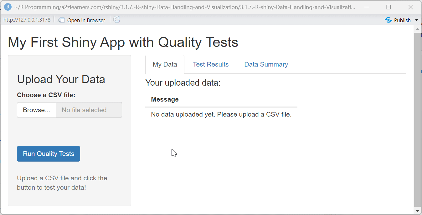
ui <- fluidPage(
# App title at the top
titlePanel("My First Shiny App with Quality Tests"),
# Create a sidebar layout (common in Shiny apps)
sidebarLayout(
# LEFT SIDE: Input controls
sidebarPanel(
h3("Upload Your Data"),
# File upload button - only accepts CSV files
fileInput("uploaded_file",
"Choose a CSV file:",
accept = ".csv"),
# Add some space
br(),
# Button to run our tests
actionButton("run_tests",
"Run Quality Tests",
class = "btn-primary"),
# Add more space
br(), br(),
# Show some helpful text
helpText("Upload a CSV file and click the button to test your data!")
),
# RIGHT SIDE: Output displays
mainPanel(
# Create tabs to organize our outputs
tabsetPanel(
# Tab 1: Show the data
tabPanel("My Data",
h4("Your uploaded data:"),
tableOutput("show_data")
),
# Tab 2: Show test results
tabPanel("Test Results",
h4("Quality Test Results:"),
verbatimTextOutput("test_results")
),
# Tab 3: Show data summary
tabPanel("Data Summary",
h4("Summary of your data:"),
verbatimTextOutput("data_summary")
)
)
)
)
)
# ==============================================================================
# PART 3: SERVER LOGIC
# This controls what happens behind the scenes
# ==============================================================================
server <- function(input, output, session) {
# Create a reactive value to store our data
# Think of this as a special variable that can change
my_data <- reactiveVal(NULL)
# STEP 1: Handle file upload
# This runs whenever someone uploads a file
observeEvent(input$uploaded_file, {
# Get the file information
file_info <- input$uploaded_file
# Try to read the CSV file
if (!is.null(file_info)) {
# Read the CSV file
data <- read.csv(file_info$datapath)
# Store it in our reactive value
my_data(data)
# Show a message to the user
showNotification("File uploaded successfully!", type = "message")
}
})
# STEP 2: Run tests when button is clicked
observeEvent(input$run_tests, {
# Get our current data
current_data <- my_data()
# Run all our tests
test1_result <- test_app_works()
test2_result <- test_file_uploaded(input$uploaded_file)
test3_result <- test_data_has_content(current_data)
test4_result <- test_data_quality(current_data)
# Create a summary of results
results_text <- paste(
"=== QUALITY TEST RESULTS ===",
"",
paste("✓ App is working:", if(test1_result) "PASS" else "FAIL"),
paste("✓ File uploaded:", if(test2_result) "PASS" else "FAIL"),
paste("✓ Data has content:", if(test3_result) "PASS" else "FAIL"),
paste("✓ Data quality OK:", if(test4_result) "PASS" else "FAIL"),
"",
"=== SUMMARY ===",
paste("Tests passed:", sum(test1_result, test2_result, test3_result, test4_result), "out of 4"),
sep = "\n"
)
# Display the results
output$test_results <- renderText({
results_text
})
# Show notification based on results
if (sum(test1_result, test2_result, test3_result, test4_result) == 4) {
showNotification("All tests passed! 🎉", type = "message")
} else {
showNotification("Some tests failed. Check your data.", type = "warning")
}
})
# STEP 3: Display the uploaded data
output$show_data <- renderTable({
data <- my_data()
# If no data, show helpful message
if (is.null(data)) {
return(data.frame(Message = "No data uploaded yet. Please upload a CSV file."))
}
# Show first 100 rows of data
head(data, 100)
})
# STEP 4: Display data summary
output$data_summary <- renderText({
data <- my_data()
# If no data, show message
if (is.null(data)) {
return("No data to summarize. Please upload a CSV file first.")
}
# Create a simple summary
summary_text <- paste(
"=== DATA SUMMARY ===",
"",
paste("Number of rows:", nrow(data)),
paste("Number of columns:", ncol(data)),
paste("Column names:", paste(names(data), collapse = ", ")),
"",
"=== FIRST FEW VALUES ===",
capture.output(print(head(data, 3))),
sep = "\n"
)
return(summary_text)
})
}
# ==============================================================================
# PART 4: RUN THE APP
# This tells Shiny to start the app using our UI and server
# ==============================================================================
# Create and run the Shiny app
shinyApp(ui = ui, server = server)
**Resource download links**
3.1.7.-R-shiny-Data-Handling-and-Visualization.zip