2.6.13. Annotation in ggplot2

1. Introduction

Annotations add extra information to your plots, such as text labels, arrows, or shapes, to highlight important features or explain your data. In ggplot2, you can annotate plots using the annotate() function or by adding layers like geom_text() and geom_label().

# Dummy ADSL data for ready-to-run examples
set.seed(123)
adsl <- data.frame(
  USUBJID = sprintf("SUBJ%03d", 1:200),
  AGE = round(rnorm(200, mean = 50, sd = 10)),
  SEX = sample(c("M", "F"), 200, replace = TRUE),
  RACE = sample(c("White", "Black", "Asian", "Other"), 200, replace = TRUE),
  TRT01A = sample(c("Placebo", "Drug A", "Drug B"), 200, replace = TRUE)
)

2. Why Use Annotations?

• Highlight key data points or trends.
• Add explanations or context directly to the plot.
• Guide viewers’ attention to important features.
• Make plots more informative and presentation-ready.

3. Adding Text Annotations with annotate()

• Use annotate("text", ...) to add custom text at specific coordinates.
• Control the position with x and y.
• Adjust alignment with hjust (horizontal) and vjust (vertical).
• Set text size, color, and font.

R Code:

ggplot(adsl) +
  geom_bar(aes(x = RACE)) +
  scale_y_continuous(breaks = seq(0, 80, by = 10), 
                     limits = c(0, 80),            # adjust this to a higher value if your label's y position is 70
                     expand = expansion(mult = c(0, 0.15))) + # add space at the top
  scale_x_discrete(limits = c("White", "Black", "Asian")) +
  coord_flip() +
  labs(
    title = "Number of Subjects by Race",
    subtitle = "Subset of all subjects, looking at three races"
  ) +
  theme_classic() +
  theme(
    title = element_text(size = 18),
    axis.text = element_text(size = 14)
  ) +
  annotate(
    "text",
    x = 2, y = 70,
    label = "Black has the most subjects",
    hjust = "center", vjust = "bottom",
    size = 5, color = "red"
  )

Expected Outcome:

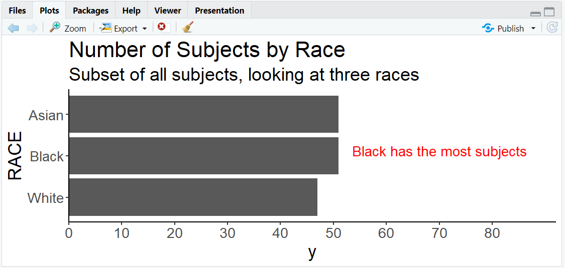
A horizontal barplot with a red annotation above the "Black" bar.

4. Other Types of Annotations

• Use annotate("rect", ...) to add rectangles (highlight regions).
• Use annotate("segment", ...) to add arrows or lines.
• Use geom_text() or geom_label() to label points from a data frame.

R Code Example: Rectangle Annotation

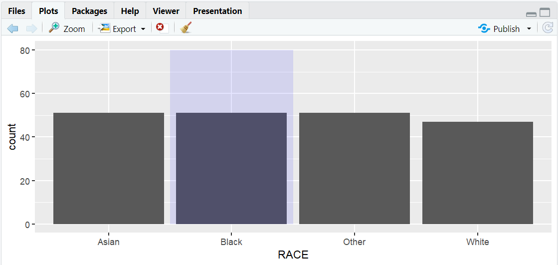
ggplot(adsl) +
  geom_bar(aes(x = RACE)) +
  annotate("rect", xmin = 1.5, xmax = 2.5, ymin = 0, ymax = 80, alpha = 0.1, fill = "blue")

• Description:
  • Adds a blue shaded rectangle to highlight a region.

5. Input and Output Table for Annotation Examples

6. Exploring Beyond Basic Annotations

• Use geom_text() or geom_label() to label specific points from your data.
• Combine annotations with arrows (annotate("segment", ...)) for emphasis.
• Add mathematical notation with parse = TRUE in geom_text().
• Use multiple annotation layers for complex explanations.

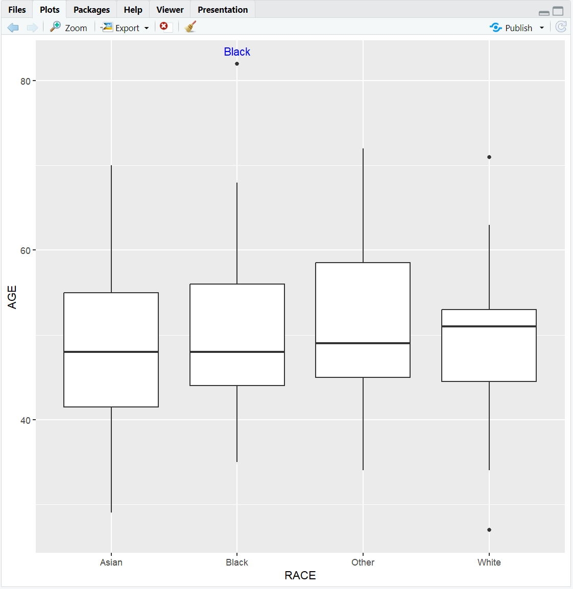
R Code Example: Labeling Points

library(dplyr)
top_age <- adsl %>%
  group_by(RACE) %>%
  summarise(max_age = max(AGE)) %>%
  slice_max(max_age, n = 1)

ggplot(adsl, aes(x = RACE, y = AGE)) +
  geom_boxplot() +
  geom_text(data = top_age, aes(label = RACE, y = max_age), vjust = -1, color = "blue")

**Resource download links**

2.6.13.-Annotation-in-ggplot2.zip